Somebody has an example or tips on how to order slices by multiple columns. For example I want to order by mean loundness and max loudness and mean pitch. I feel I may have to normalize before…
It can all get a bit fiddly, although I made some abstractions for a workshop a few weeks ago that might help, linked in this post Using slice and ears.fade -> poking into buffers - #8 by weefuzzy
If you use those, then you could use fluid.buf.pool and fluid.buf.stack like:
loudness–> pool   \
                   stack
pitch   -> pool   /
and from there into dataset?
Hi, I noticed for what I want to do I can’t use bufstats~. It’s way to slow if you have many slices. I guess it’s all this repeated buffer handling. I’m trying to calculate the stats myself currently with a js. Later I want to normalize and do distance calculations. I came up with some questions:
- What are the derivative values? How to calculate and what do they describe?
- How do I absolutely normalize skewness and kurtosis? Are they in the same unit as the feature? What is the minimum / maximum of it?(for any input) And is it linear?
Here is the script for the stats per slice output. Only kurtosis results seem to slightly differ from bufstats~ results. (Couldn’t find the actual formula on flucoma github code) Hence my question 1, I was wondering if I should add derivative calculation when I understand what it is…
outlets=2;


function get(sourcebuf, slicebuf, featbuf, featbufchan, hopsize)
{
	var source_buffer = new Buffer(sourcebuf);
	var slice_buffer = new Buffer(slicebuf);
	var feat_buffer = new Buffer(featbuf);

	var numOfSlices = slice_buffer.framecount();
	var onsetArr = slice_buffer.peek(0, 0, numOfSlices);


	//post ("\nnum of slices: "+ numOfSlices);
	//post("\nfeat frames: "+ feat_buffer.framecount());

	//for every onset
	for (i = 0; i < numOfSlices; i++)
	{

		var onsetTimeInSamples = onsetArr[i];
		var lengthInSamples;
		if (i == numOfSlices-1)//last one
		{
			lengthInSamples = source_buffer.framecount()-onsetTimeInSamples;
		}
		else
		{
			lengthInSamples = onsetArr[i+1]-onsetTimeInSamples;
		}
		var start = ~~(onsetTimeInSamples / hopsize);
		var length = ~~(lengthInSamples / hopsize);

		//post ("\nslice: "+ i +" feat start: "+start+" len: "+length );

		var featArr = feat_buffer.peek(featbufchan, start, length);


		// skewness
		// kurtosis
		delta = 0,
		delta_n = 0,
		delta_n2 = 0,
		term1 = 0,
		N = 0,
		mean2 = 0,
		M2 = 0,
		M3 = 0,
		M4 = 0,
		sk_g = 0,
		ku_g = 0;

		var mean = 0;
		var minimum =  (Math.pow(2, 53) - 1);
		var maximum = -(Math.pow(2, 53) - 1);
		var stddev = 0;
		var skewness = 0;
		var kurtosis = 0;
		var median = 0;

		for (var j = 0 ; j < length; j++)
		{
			var value = featArr[j];

			if (value > maximum)
				maximum = value;
			if (value < minimum)
				minimum = value;
			mean+=value;

			N += 1;

			delta = value - mean2;
			delta_n = delta / N;
			delta_n2 = delta_n * delta_n;

			term1 = delta * delta_n * (N-1);

			M4 += term1*delta_n2*(N*N - 3*N + 3) + 6*delta_n2*M2 - 4*delta_n*M3;
			M3 += term1*delta_n*(N-2) - 3*delta_n*M2;
			M2 += term1;
			mean2 += delta_n;

		}
		mean /= length;
		sk_g = Math.sqrt( N )*M3 / Math.pow( M2, 3/2 );
		ku_g = N*M4 / ( M2*M2 ) - 3;
		skewness = Math.sqrt( N*(N-1))*sk_g / (N-2);
		kurtosis = (N-1) / ( (N-2)*(N-3) ) * ( (N+1)*ku_g + 6 );

		//post ("  mean: "+ mean +" maximum: "+maximum+" minimum: "+minimum );
		for (var j = 0 ; j < length; j++)
		{
			var value = featArr[j];

			stddev += Math.pow((value - mean),2);

		}
		stddev = Math.sqrt(stddev/length);

		featArr.sort( function(a, b){return a - b} );
		// Get the middle index:
		id = Math.floor( length / 2 );
		if ( length % 2 )
		{
		// The number of elements is not evenly divisible by two, hence we have a middle index:
		median = featArr[ id ];
		}
		else
			// Even number of elements, so must take the mean of the two middle values:
			median = ( featArr[ id-1 ] + featArr[ id ] ) / 2.0;

		outlet(1, i, mean, stddev, skewness, kurtosis, minimum, median, maximum);


	}// end loop over onsets


	outlet(0, "bang");
}
1 Like
Hi @11olsen,
Can you share your Max code for the bufstats~ usage? It really oughtn’t be slow at all, so I might be able to help with that, or spot a bug.
As for the questions:
- The derivative values are the same set of statistics calculated on the nth derivative (actually nth-order difference), i.e input[n] - input[n-1], input[n-1] - input[n-2] etc
- In reverse order
 No, they’re not linear w/r/t the input: skewness is cubic and kurtosis quartic. They don’t, I think, have units but if you took the cube root of skewness I think you would be back in the same units the feature (beware negative values though).
Truly absolute normalization is tricky because these quantities are to do with the statistics of a sample / population, so there isn’t a universal thing here beyond what you know about the limits of the quantity under measure, i.e. the maximum conceivable skewness would be ± the maximum range of your feature cubed. I think that would turn out to be a uselessly large range in most practical cases though, because your sample skewness is going to live in a much smaller range.
One approach, if you’re taking lots of stats of slices anyway, would be to take statistics over the whole buffer (like a population) and use that a basis for normalizing?
Hi,
- Ah Ok, so it’s kind of a variance stat. And second order is the variance of the variance and so on. And how do you get n-1 for the first frame?
- If I fill a database with features I need fixed min and max values for normalization. Because anytime I add more data later, the min / max values could change in the database. And for distance matching I need linear (perceived) ranges for the features stats. Frequency units scaled to 0 - 1 for example make no sense, but midicents do.
I can test a big example database for min / max values but it’s hard to test for linearity of feature/stats because I have no completely equally distributed (perceived) test input (audio slices). If I see a peak or ramp in the slice distribution over the feature It can be a mixture of an unlinear feature range and unlinear input sample distribution.
For example the loudness stats of all slices of the package’s example wavs:
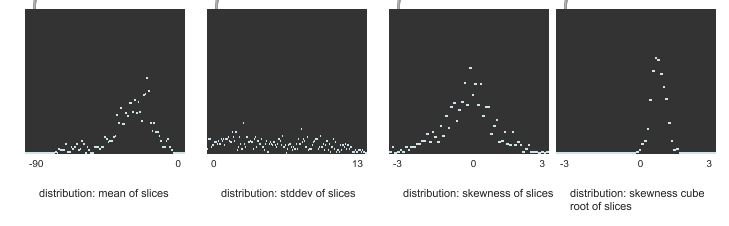
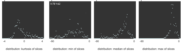
While the db values reflect the perceived distribution of the slices, i can’t tell for skewness or kurtosis. The cube root only seems to shift the values.
Here’s the patcher. at the top load a soundfile > 2 min. When finished at the bottom you can see the slower method to get the slice stats with the bufstats~ external.
2 Likes
Cheers!
I’ll look at the patch in detail later, but from looking quikcly my suspicion is that your problems with bufstats~ come from using @blocking 0: it happens to be a pathological case at the moment that running lots of small slices across a single large buffer in that blocking mode is sub-performant at the moment because the whole buffer gets copied each time. I’m reasonably sure that just using @blocking 1 there would improve things (at the cost of a little beach balling).
Meanwhile:
- Yes, the derivatives are indeed variance-like, although they don’t describe deviation w/r/t a population mean, but as a function of time.
- It’s quite possible that skewness and kurtosis don’t add anything of value to the data for your purposes, especially if you need normalisation in absolute terms further down the line. You could cherry-pick which stats you want using
fluid.bufselect~with the@channels <list>attribute to select just particular stats.
Alternatively, you could look at putting all this stuff into afluid.dataset~and then usingfluid.normalize~to adjust each feature independently.
This is only experimental to see the maximum amount of data I could get for a chunk of audio and how long it takes. I really need strategies to then find the most valueable features and stats. Before in JAVA I only had a mean stat for every feature and it was already working quite good. But I want to explore the usefulness of the other statistic methods.
Btw: @ blocking 1 mode is a bit faster but still can’t keep up with the js.
I’ll check fluid.dataset~ but I don’t think that it fits.
Thanks
Hi again,
I’ve had a closer look. I think what’s causing problems speed-wise is that the stats buffer ends up getting resized a lot of times because each feature has a different channel count.
I think a quicker approach for this is to use bufcompose~ to stick all the features together in one buffer, and run the stats once per slice. We can then use fluid.bufselect~ to to cherry pick which stats we want, or fluid.bufflatten~ if we want to squish all stats for all features into a single datum per slice.
Now, in an immanent update we have compiled versions of fluid.buf2list and fluid.list2buf which make this whole workflow much easier. I’m going to dm you the externals so that you can try out an implementation of what I’m describing above. Am I right in remembering that you’re on Windows?
The fluid.dataset~ can do essentially the job that the colls are doing in your patch. YMMV of course. The upside of the dataest is that there are objects to do normalizing etc., as well as other goodies. [coll] is very convenient though!
This example spits all the stats organised by feature (feature 0 all stats, feature 1 all stats etc.) into a coll.
Max code
----------begin_max5_patcher----------
5346.3oc6cs0biaqj9YO+J35JOrmsbzh6W1mx96XpsbQIQayrThZEolLmj5j
e6aCPJIdmfTjxZlhNUr4PHJB7gutQCz.c+We4omWG+8fjm89u79p2SO8We4o
mr2xbimx+2O87N+uuIxOw9wddWPRh+6AO+RVYoAeO0dezJDFSwXujfMw62lb
9Cr+zt3SoQAo1GGme2vs1GJd8u+qDM57mM6Cl9OODjUid9Yu+m7hN3mt4iv8
u+5wfMoYkJUqPvOTrfiPBAUJdwipj1ahPDphgUbo9EOLljcSrhIkLpVodwi.
26x2NTIC2etNRL26e8kuX90K2Hp7Ki.OThIDOXpUZ6OXDWSQTBzzkPe0TC.6
C9CnxWq8+e3AuKDd.MddqM92hh8SGNBfzqnvOLNgBc8LjjBLBzL.AqOklFue
.M0KvxA+i96BRCN9Zvd+0Q1FLpMXXs+926DEnYMXAUQwHFkvnYsTKzPoRk.g
QR3dLKFvZCCvSGM3WAZf6.iTNwb.hLmCvnLPDfwPjYhCzR6eygSahh27+N.L
PbCX.Qly.XRJCyoRto4RVA+gy6tQi+Taz2hvOVxx54YbLFozThsUmcSDWpLL
BtQX3NhAodqM+WyP.sIHf8bmB9uT4u8nHffXZMgJLBCJFHJHvVpAnE.jEvJL
A6fjvDBHG7fNxsu5GE85t.+8IulF+5l3nnlQHTSHD84Nj90qjUaxDngogw7E
bNiI0bswj.Fqmlbw2Qvw7FZdK8omeKLJ3aAGSBAE9W+zO8r+gCEt8SEdDC77
6w1uH0KWtU39ragubqiAeK7xW60a6eDZpoP67zQKe34uKNyTLeOwaCNt+T3k
NKaOUdcx1mrGFfI4f+lrG1z0ct3qfG2hI.DB+FSjXyeUH9UHB5ye2HQGrsPm
CvTODrOb+giAIA6S8Syq7WJdava9mhRe8s38oIg+osFfMLtFJ+s7ZXiEZZC1
p++8wP+nKMf2OFtMduoRTpqvb6yuNP6fUlGWpwX+D68OzvCCLM.VZovDnQdJ
Ys+QSOU9v0jyElFGGUtnKOWTvao4EeHb+9JnXZ7g1K7X36ezwytNFJbWWe21
RRd8z9rReE3Doul3+sxncJHWlK3V9q+696C24mFjFl0EPPWJLyjkOR1bzHFW
r8lUx2Znjs.IeSveDtM8C6KpHY.93gGNShd9Ru71v2CRRKeuT+2SJemjz+YF
nW3VmVmKD+ZZvtCQPqHSFH78yB2WjdSRBSRS9H9ORxK5LkqHTbc9REEuKpOr
z86blBkUNdL3sfiduEGWrzFG1rpVQZwmn8oMzlZSNhZDOfouY9COa3.TAYkl
MN5oyCKjqvYjPxuGltZSPTz5BVKzPSm0bSGW7IZQGSinRDzWaFG8x+Wp0dDH
AVk0nJe8MqEpUf0pSkxEl+HTYHKLorxPKLBXFpxosB3UpFWzTNgcDkFytL0b
8o2.t4e6Yz8kzdeDok9HNuSBZl0cUsooU6ZxUlCiTAewZAhfHDrDarpWv5m6
huuP1afJmQBaL5L.a.6SHoJgPHYTDCrRBFzW9v.aFqA6VGXKJBHRT2ZAaUVu
AvhoWAVLhjLgl.SW1rhQBj4dv7GwJFmgIDNypqj2KvUn.yPtaeMy7hW8SSOF
t9TZ1HJOUCyfgP2st7P4Y0WnddwHQwkBtzuLy8P+db39AOBEQnuswnZnGgCp
U4v+VIoZMiqTJSegt+djobzqtFPGMBXRcavDlSrhxZ4JpRxkBBAvGDEqu+Cr
2AGJ0Kx6Oi1DE3e7xziaeJx0QIQuh54e6NqdLGbn7URsFqgQW3DkliElICge
fTOdZe5UaVcW6nn6gfC2WxXHy+zMDiZD3D.sCF+kxwXkRZWlgdAL98hos1KZ
vC8RJL85tVLFWoUMINddcWdDnUuEcJb6JvjEhwrXnSUJjd+VR7oiaBbwBFba
VvzMqyZCdupznYSKg.FtnoLgTi4HtBSMKtCR9vnS6aAe+vQOPx4e+WdC68e5
wwj+wvQL5MNNYNZQAEYJMSwYHJnFiJU3GTFmgckFr+uuP2rTMueaKLe+v810
S5JCz627+dXhGZvCYfoJmDnuXSsq.MSCFgHPTA7KBUxPRiuUT5GOf1BfFX1B
j4vYNlaVP12B7MKuXxHvVwLgsvz4XDIQPA.UnMdv0rnsh6K11kEdvK8Miy6R
79E7Hj042lrNgpVgAEhJgBA.jjCipvnjUDMCCSWQJQHt1bSI49pkrKHCHdGS
sfFfYu3kQNFLxglDsjvreWgEXXzDgfYlYmw4.Z9CyPJ+aE7b5.PGBxg0MXTj
KDdkvLALslKgo.CSG99OiqdlVwvM1CLZs+UNv0wcEpUHBL4AAXLrv3mMy7GD
0PxGhgF9ynbK8RROF3uyiLBnic6PWtMxfRJkBA1GqnJDVSktZwB4NiVm1G9+
cJX3XEROYXEX1KUqoHvfXEBl6kwniGIrJ0CMFAQjxoIo5FHgYzUXJ0LuTPBT
wPF4NtCJqv2u0QyiNbs6na1aOYKeNeEQHHHlfvAsVXisUNQgn220OeS792hO
tKyP0QPoPS3Zni01cQSiqgNFKM1RHwvb7A0DfrI4Agn8dPpYol8R72cX3V2q
0tsr5Ntxj4TreXV7ijnvMkmSTT39.6xvUk14j3qlc6qHBGUGIMlebeT6a+VG
9JaKI8OIQWZ3lMxKkhjZDGDGewrMmx1ai4lMXVnCZFjzI4BUxAr61Eru71Kv
V+2uM36swDutSRLLhV1U.1Fgo7lA1bsZYPvEXxqb0tvJgT3SZjKq7AiOtMau
J4lWgmw5Fq85FddpaFWB3gcntYMY0T4lw5Awg5g0UOyV8vZroS8UY034EOPO
.8KNiGF+HOi0Cty8K5Ysdnbtdvqwn2Et8.X8ZZtROvrGiYQTyNsTx3Lk.510
XrY0ATnVJZ1ZXrA0vPyZ8vIERz4ri9hXkC3wbJ.ZWrS2TDPqqxnBgivjqDUW
aJXpcTARQ.qy4foALjci9ZoeMT1r0L0NquaV0+SQCEtmm5Aw85AeVECTNWOP
yd8vI0BjYsdfbtdXVuAymblpGTW6WP5YGOPNiGyU8PybtZLmpOz5AgFtXc.F
zYWa43x0O2PYyYCyMZ+bJ94LoeNo7rgYJ5roBf5rnGaVGhf57TUnsK6ccUAr
GFgVVVfK6hbLtxoP35gdo4ps+lMA6S2DGkcxg9pGH.Al.wASsythxOeEyHYU
YIPV+doGELGWxrOfRh3lMUo4JEihq+nl0Ky9vuFt2bJmBN+kfdovup+BeKLJ
5xKsoc454UA542O5uMzrNLE2sqkpuDMBqElWEEoUHV1UvspWeyeR74GUvgmv
74ElejYWk05a9IImeRFSZePlhIQX6URp4nkU6472+d94ARV5zGX1ytwGhOd4
vQshpK8bmRiuz3Kt9MWOGWkXzkvDJgyzVffctIRkmumlUjk9RAgiiv6p94kw
n9F3dgEqEMIbUm.W7jXLqT3ROHFaZqYebD0rdfnURysZ3AKd5P9p87gzkng1
HEXIXZofIwEuZQz3mDQiVNUMes7fcyqXymifSAM+WuhxIZ1MK3bg9oyoeKio
rH3LKBNKi4rH5rH5LFQGxhfyhfyhfyvEbnKBNKBNKBNCUv4dMdyvX+KK+0xx
eMYL761jQVHwKj3YhDSWnvKT3erovrEJ7BE9GQJ7GAQGLAVxWi7WGD4t0DWX
SWXwWV185Wg6xZYZsBOW49543c1LiA67+tnPzobDhvYBdvbjwVxsLmb2ozKN
WbK+W.ZMVw0YGbpb3K5FdJALLhw6Nk4zFgV78ppW6Pg6Hs9SPII9pV8yZ3pe
UO55jJEIaDj5W07iNJUyyghRWnB0kTGNiH6P.MJ1rs+mAzXjcwvXZy5hMYL4
hQ7110Sb8kc9M0W7c6uFSXNss.m66Qwq8ipDoRu9XYQp2W6sATOZp9kqrfoJ
pOuId2ZXz1WaHNi3PfAWPddzgC+lBIzXkYgOwHLV.ZE0JE1DP3ozkXB84WXS
wDZN1BPBJYIjPuDRnWBIzSUHgt5nfsDE7qpUjo5I3CmkfOxCdgtbhXw25Ih8
gIhtzSXmyoyqtfYO3ZYQxKo79F1HNC+MAIQA6eO8iDO+8a817g+98GCh7rGH
8wbL0aicQ6ickESqwDa.3SmE2k0OB3S9A2OK9QT.l.TJ9s2RBlTXhzCLoTYw
1FKKRStunT2AylH+QDOMXnoRxhvUvTRHLDCthvwlPhYNZc2hfMcQi5fy3D0n
bfbrw.hAMKPrXYExLwI0C.2.raCLvYq2vCew8DH.cHHZQsTCB2rfUXJgASXl
ijTv9b9iSncGDdB1DFk3gGr7CUNEgZLKJg0VoEl7QJBYsMXTpUnSv.1XTd.t
GuBCZTHRgh.bHASBfj5AJzXstaaZZIN7PcLhD6BTkYZnP+nEIdNq4omHUTaZ
eH2Z3zL2TY1JFX1LiwYTjFivxGKT5bjwxsf1ZaRbSYtkfbMnCi3RIlnkDrfg
MoHgGIjaTot.JdRnUDI0rO9zDJBFXCi.LxDzvzONV7jFCy1+rsxSnQxkCVqM
kaGP4oiMqMPb4iybIfOnW17sFr8ej9r+KOEqQnrqs56m8ecEhdGQrLlHmFgj
7f67iSHkEroII9Xp2uNba8HSfQM43xCosdIm1MbLgd6XBMmq.5NovnLbNXiG
XtGQCbFA+m.qgI3oi3..RMqgu6i5zkIedlL9jwcYYl07pYE5GtsejaMffmM4
Ac1rvQtLWypegAs5w4VbMTatGpxi2jahZwUQc3tn9cYTatMp5lmoO2G0nKjX
h1Sqns5GIG7kjK9SpWeJ4nek5v2Rt4eod7wTu9YpWeM0i+l52mS852IG78jK
9eZH9fpC+P0qun51eTc6Spt8KUm9lpM+S0rOpZwOUCzWUN5upl8YUUUNUUrW
q79Tv2zZdTNQL0ftcVkRKFGmkUezNWAjFyOSsudZjU1rEd95y27nicXNd4cM
SoQJmYfsxDZ6d7xZXJtWLcP3GEloOixPJtjHjToVJZc5+cXuwmGZ1Vfxt6Eo
qFrh5GVaZg55CdI.FV2d2eb3pf8vueL9zgtAVR6.q1MbcPTVpXEVQXHMmvzX
ovDxRennr0mmdEucFjVN2CMLc.poUE.VPqyQ4+3nAHb+aw+c2fotcvTzKXdY
YUOm8oubCWtnoLyXqy+Cl3GWQu9i4D8RDnFVCxrr+8OD5PxW56QqBg6dOTsE
9tc+3JyzO2D3xP+vfsgkyqnCSOBch0ibcyX9CB5k1u4scvKItacqKvXSIHhG
CTrZxiXfVrNQCWkgOLT66Lt5nCpRgsrC4ZYWxMiPZs8OX29nnFlVyrpNjKY3
b6kXnreHtCf3oF.KutJ0RBG0w0lhHnMft0CZrUiKnmm7eSwFzJQo3A0wO1JX
8facG0PxmPEjTMp61Q8i9IU+bE+ZlMTInGmkmwnlMZgFSPLofXxP8lC8nYCp
Hatv6bqlNfVs5SnWYHrZyBDc+k6jUC90cTCEeVUP5idEz49XzmUMzUcWbWzM
PPpUv.oW+QYxj4L0JNWnEXNRHPbLyjS4DBqphFJ7diB3gqg79VAQCgHg+Dpg
FwK0Ppf39HRTXTFTs43qTqHXIhQTBJUnzJaRyljQjpW3mQ+z.Emb1FP2NslU
cnYemZyptycTd8oKeS18I4bLmlylNQmUOauy8lbMb366AAxo83Z00.qwYrPr
qf.yrupjbMioEHLVRYFCuVQYli+IgnXRN2J07PjN4yO5JMkWzusrNIgdi6Oq
ryrACqWwDJJGywTLSRMavSt59l+I6bmqQF9NGou8dtqLslvlGnMxl+lMcses
ZEcn8lRlcEfzhUbiWAMaqZlRwMl8v3q.yZHHXBPBMGCyM5dl9g6TVLHcDm.F
xstIzw.hPoflPFniRvALwLUQABF1liUBBUAigqj5yq6xCxYZHxa8H1Kf8eXx
bZ6mmeTMIhULfZA3lRRwTEi9Ir6y6hRYLxII0+XpYOV6MlcYKgLI5p3lCEb0
MpOHdBZuXLByPxPLSHH4QYiTZ7MgGYDajR8jcPfaRDjgeXDAujDq2Du6PbRv
e68aEro1wyJBssMWI1I6xt5nR2vTNOeZsv3kbIkXmoBXbrfRzffqjn.gYiWz
tehuiL4VKt0yHR1Y0WuRa+w3.QMCj1+gNUVSbMcQa4WcmwOMNfvxXvqnHIkp
Pbklo3lylkL6.TTun4J0tRkCsgMSoXVjiIyNqUbyVBbKqdfbtdLa3A08DZ2r
limotld+tHhLS0CxP6W5P.jy.yCpXWJb0JyF8QK0D3ObsY504hpMT1r0NcWN
XdwamkCvyZt818pQu85X6.0XBLGeoFaLpFi3BEwL217b2Y8xJ8MFeba1Ii.M
OMVmk4kyIjicsVvm6ZgaxAyYsv0QGoy5fizgTKlqgFcVC7rNvH0U147pdzU0
RMLL9EkH34AfX0RhwsYP2b1M4rfyblw1snuKJQnyoBUmyEuLzbJ9xbDKXyIu
f4t40yZ0f67nK74tZ3FZLui36ZJReVSZ0TWyW7L0rNSTmGgg4PlydIn6Njft
a4UbtvJBF3ml7ZT7osdYWdHDp04Wmb..q7q281lM4Wt4iiw67O+UUxmibmCW
uHZqgq2gGpdQ1ISpHqHDohiDXtVBSw.mEwzZNR8RJfh1OQ4k0JCTqxwyg1FL
aojkjsthBELcpVGnyuKAwk2kjNEuKYoA2Z0fmo6cQ5scwmr2U+XnXRdWbmdW
xq1nbCuKgyuqatcovN8tXSBFJc4colDtgxo9K0jvMTN0eoQ03FYprpDXHLul
JABhJA.hFB7CsGvGpFnGrCllcHzqnmrdJ1IS6dkf0eNLL9jpyHSnNCOOQzTN
h3rMBslaHFWFZXbINmwjzbZNOPzdNfnk7+vEaptgDjS92QKobgxoaghBVMkt
UmIp1XRtpcjZIGYRUcg59HQcKzKWKAoNkT56Cotf1yqWYR.PrQSpuPWzWxpT
K5iWH04j5Ec0Kz5e9n0jER8Bo9mMRMcgTuPp+4hTOW5ocmctrbEKKWAY1LBd
grsP1pP1nKTsEp18gpwVnZKTs4jp8QPzASPR+0H+0AQcOJ53R28slp66JM2e
ysqRIIamEe5OE16Z5qenot9IoAW3HT0bSdvok9IoZUZaxzC05NnXYvoX9Qld
4GoZroR4RWcekkNbqWrXvtyA1UeoI9gwrxbLeKY+fu7u9x++Z6GKu
-----------end_max5_patcher-----------
Hi, I thought about stacking the stats before but discarded it because i was thinking it won’t work if I want to have different hopsizes for the features. But I can live with this. Thanks for patching this together.
Yes using Windows os currently.
[coll] is only in there to take a quick view on the data. In the next 2 steps I would normalize / standardize stats and save a huge amount in a sqlite db. Then I want to be able to find the closest match to unknown audio input.
fluid.dataset doesn’t look like it can hold/save/load hundred thousands of lines (it’s just a json file), or is sort and searchable.
Even with the improvement, after comparing the times I would still stick to the js to get the stats. When I process a lot of files this makes a difference.
130 slices - bufstats~: 3.1 sec js: 0.3 sec
900 slices - bufstats~: 21.2 sec js: 3.7 sec
5000 slices - bufstats~: 98.8 sec js: 24.5 sec
I’ll DM you the compiled versions of the buf2list(2buf) now, as my numbers are very different! I’m seeing the bufstats being an order of magnitude faster than the JS when I stack everything. I guess if you wanted to avoid that, the key would be not to reuse the same stats buffer for all the different invocations of bufstats so that the resize operations were reduced.
The dataset should scale up into the 10000s of entries and above, but indeed the querying might get clunky, especially with this many features. I would The fluid.kdtree would comfortably outperform SQLlite at lower dimensionalities, but its performance tails off markedly as the feature count goes up.
1 Like
Hi again, after testing again today, bufstats~ is much faster (takes less then a second for 5000 slices). I don’t know what caused it to be that slow in my test yesterday.
That’s a relief  Many thanks for letting us know. (I suspect that the compiled list2buf2list externals make quite a difference, as the original abstractions are pretty inefficient, but a 100-fold improvement is pretty dramatic!)
Looking forward to hearing how your project works out – I don’t think anyone else has gone down the SQLlite route yet, so it’s really interesting to see what affordances this gives.
2 Likes