Bufstats~ on short buffers?

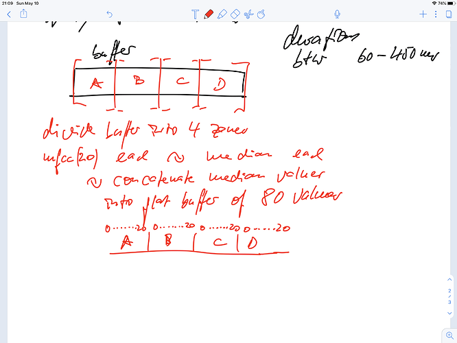
I want to experiment with some kine of ‘dynamic’ mfcc. Each sound is divided into four equal chunks, each chunk is analyzed with 20 mfcc factors and median is taken over each one. Then all four analysis are combined into one flat 80 buffer. I hope to get some kind of a fingerprint of spectral evolution which is more informed than the derivatives of mfccs.

The problem is that many of those sounds are short and by cutting them into 4 parts, the individual buffers are now shorter than my fft settings. Is there a way to zero pad? Or some other genius solution?

Just tried to add the patch with copy compressed, but it exceeds the discourse message size.

https://drive.google.com/file/d/1M3dC5sfjco3sF5ivr8JIn4Wq7Pv0gDCy/view?usp=sharing

there is! The fft settings are in effect WindowSize HopSize and FFTSize. The WindowSize should be the size to fit your data if it is that small, which can also have the same HopSize, and then put the fftsize at what you want and it’ll zeropad it.

You could also not use stats at all and to the same. It really depends on time and spectral resolution you want, and also understanding that you cannot get a lower frequency for real than the WindowSize, however large you make the FFT after.

So case A, at 44100, you put the values [4410 4410 8192] and you analyse for 17640 samples (4 x 4410) you should get 4 MFCCs out (times the number of coeffs, one per channel) so your 80 values. This is 400 ms.

Another case, same SR, you put the values [2205 2205 8192] to keep the same FFT size, and still process the 400ms. You can average 2 points per 100ms as you will get 8 MFCCs.

Another case, with [2205 1103 8192] you will get 17 frames of MFCCs, and you will have to deal with what you do with your overlapping ones… or you can do the math of knowing which frames are fully in each section. The helpfile of fluid.pitch~ makes it quite graphical what to expect in term of what is what.

Personally, I would try Case A first, as the windowed FFT process is already an averaging one, blurring together what is happening during that time window. You would get better low end response, but again, it might not make much of a difference. Also, MFCCs are getting less and less significant as the coefficient gets higher, so I’d try with the usual 13, but I would always scrap the first one, as it is strongly correlated to amplitude, and less timbre, but you might want that feature.

I hope this helps your explorations.

p

This is brilliant. Thanks so much for those details. I can scrap all the cutting into 4 buffers and just ‘hop’ through the sound in 4 steps. Then I don’t need the stats either and just flatten the 4 samples * 20 channels into one flat buffer with 80 values. THANKS

1 Like

Now that I got something working I like much better than all the attempts over the past weeks, I made a quick video to talk you through. I will also put a link to the patch below.

https://drive.google.com/file/d/1uXVCcLE7lYC1wS8RvQAIwXvQSaNnGVed/view?usp=sharing

the patch as max project
it uses some bach functions
ht.fluid.mfcc.test.zip (37.9 KB)

Permissions not set for anyone viewing?

It would be nice if sharing files through discourse would be easier…

Try this one

https://drive.google.com/file/d/1uXVCcLE7lYC1wS8RvQAIwXvQSaNnGVed/view?usp=sharing

3 Likes

That’s great @tutschku, some really effective results there and a really useful finding - glad you’re making progress.

Hello!

This is a nice explanation indeed. And very, very convincing!

One small detail: if you do not enter fftsize (so frame hop -1) the system will zero pad to the nearest exponent of 2 (which it needs to do anyway, you cannot go smaller than that)

Another note: the peak-uzi for flattening is the best way so far but we are working on better ways now.

Finally, some ideas that might or might not make it better:

  • replacing MFCC0 by loudness measures in parallel
  • slighting harder: having the first 3 frames at fixed duration (let’s say 20ms) which gives you a comparable onset in time definition for the first 60ms, then average the rest of the grain as the 4th (which is what I do in the APT patch)
  • something else: comparing normalized and standardized versions of the dataset should help when you get to timbral spaces much more different… but so far my experiences have yield mixed results (they are in the APT patch too)

Congrats again, this is very potent. I will certainly try it with my sounds later today

I’m happy to brainstorm more, or explain more, whenever you want, or if you hit a ‘problem’ in your current implementation. If it never happens, it is not a problem at all!

Thank you both @weefuzzy and @tremblap for your encouraging comments. Is there a source ‘mfcc for dummies’ you could point me to? I’m still very vague in my understanding of it.

  • replacing MFCC0 by loudness measures in parallel

I have heard that before from you - is there a good explanation?

Some guidance with your APT patch would be nice - it is cryptic :upside_down_face:

  • something else: comparing normalized and standardized versions of the dataset

again, those are concepts which have not trickled into my understanding

It might very well be that you presented all of this at the last plenary, but those topics need time to chew on - not just listening to a presentation once.

This would apply to sounds which have the typical ‘note’ concept. But I’m interested in short sound with some spectra-morphological evolution (gliss up, down, reversed attacks etc.) - hence the equal division over the sound’s duration.

I’m sure @weefuzzy has a plan for those in the learn.flucoma.org platfom. He explained it to me very patiently one day…

Good? I don’t know… But what I noticed, from my use of them and from the wisdom of my colleagues, is that MFCC0 is a linear representation of amplitude. In the help patch of fluid.mfcc~ look at the left bar of the multislider and change the volume on a square wave, you’ll see that it changes linearly, which is not very useful

So I prefer loudness for 2 reasons:

  • it is in a log scale which gives the distance in dB a more perceptual value than the distance in a linear scale (where the top half of the scale is used for 6dB and bottom half for infinite)
  • it has a perceptual filter too, which gives us a better (less-worse) estimate of how loud the sounds feel.

Let’s do another of those shared meetings on APT in the next week, I’m sure a few more people would want to have it verbose. The good news is that I’m reimplementing it with an interface that would allow more dynamic exploration of its settings…

I think more in spectromorphological / Gestatlic ‘events’ than notes, and your short sounds were presented as such, but that might not be what you were looking for.

1 Like

The 0-th MFCC coefficient represents (something like) the overall energy of the frame. It’s often discarded in order to make comparisons insensitive to differences in level between datapoints. Where one does want to capture loudness differences in distinctions between datapoints, better results (in terms of matching what we hear) might be obtained by using a metric that is more principled, psychoacoustically, than the unweighted energy, such as from fluid.loudness~.

As soon as we are dealing with the ‘distances’ between multidimensional datapoints, then the relative ranges and distributions of each dimension begin to matter. If each dimension has radically different scales (e.g. frequencies covering the gamut 20-20000 vs amplitudes in the range 0-1), then the biggest ranges will swamp the smaller.

So when to choose one over the other (or neither)? It’s pretty hard to come up with complete guidelines, because so much of this is in It Depends territory, and we don’t yet have enough notes on musical experience to make confident pronouncements on what the musical consequence of different decisions might be. That said:

  • Normalising, as in min-max scaling, is certainly more easy to intuit, as its something we’re all pretty familiar with.
  • It can be particularly useful when one is interested in the distribution of data in relation to absolute maxima and minima (e.g. pitch limits you come up yourself)
  • However, when normalising against the intrinstic min-max of your data, it is very sensitive to outlying values. Staying with pitch, if most of your data is, say, between C3-C4, and you have one G8, you would end up with the impression that most of your points are virtually the same, which may not be desireable
  • It doesn’t entail any supossitions about how the data are distributed. This can be a downer (as above), but – becauase it’s easy to understand – can be useful when used with models that also don’t rely on assumptions about distribution (like KNN)

  • Standardising is different in that it uses the mean and standard deviation (the average distance of points from the mean) of the dataset: things are centered around the mean, and scaled by the standard deviation.
  • As such, it’s focused wholly on the distribution of the data you fit against. This makes it a bit more robust to outliers.
  • It also implies a (mildish) assumption that the data are normally distributed, to the extent that the concept of a mean and standard deviation make sense on the distribution at hand. Often this is true enough but by no means always.
  • The units of what comes out are no longer simple to relate to real-world quantities. Things will be scaled in terms of standard deviations. If the data are normally distributed, this means that you can make certain assumptions, e.g. that much of your standardised data (68%) will be in the range ±1, and almost all (97%) will be within ±3
  • It’s pretty much obligatory if you’re trying to compare variables that have different real-world units (not the case above)
  • and for models that do rely on normally distributed import (don’t think this applies to anything we’ve done yet), but here you’d need to verfiy that this really is the case as well

So! Where does this get us for something like MFCCs being fed to a KNN? Here we have, often, 12 or 13 dimensional data, but whose relative scales vary a great deal (and aren’t easy to predict), and whose individual phenomenological significance is pretty opaque. Without any sort of pre-scaling, all one cas say is that the coefficients with the greatest range (often the lower ones) are going to dominate any distance measure.

Conseuqnetly, I’d certainly reccomend doing one or the other, or at the very least inspecting the ranges of values. If there aren’t problems with outliers, then I think normalisation would be fine here. This makes it simple enough to then apply a weighting to individual dimensions to experiment with how that affects the matching vis-a-vis your hopes.

(I say ‘simple’ enough, but do realise that we haven’t made useful interfaces for doing by iterating over a dataset yet).

2 Likes

Few notes on the amazing reply by Dr Fuzzy

2 keywords in there:

  • might (MFCCs distances are strange on their own so putting something sensible in the matching, on its own scale, might actually be worse)
    and
  • unweighted energy (the linearity of it, the enveloping, the size of the envelope, etc will influence that number too)

but this is what I explored manually in APT code, to some success, but opening a huge can of worm in my poor little brain. But this is where it is fun - trying to get better results and follow strange intuitions…

I’ve found surprsingly few explanations in the wild that satisfy me. Plenty that tell you how to make them, some that explain it for data scientists, but nothing that really reflects much on what they might ‘mean’ for arbitary sounds, from a musical perspective. I think a complete physical interpretation probably isn’t possible, but here’s a couple of possible ways of thinking about them.

Way 1: Dimension Reduction for Audio Spectra
Possibly makes most sense for a black box approach, we can just think of the process like we do another dimensionality reduction techniques that do something magical, but at the cost of directly interprable outputs. However in this case, especially tailored for applying to audio spectra, and warped in such a way as to coincide with human auditory perception, in principle.

This isn’t too outlandish: one of the steps in obtaining MFCCs – the step that gets you from the spectral domain into the ceptral domain – can be thought of as an approximation to Principal Components Analysis (for which y’all will soon have an object), which is often the first go-to simple dimensionality reduction technique people reach for.

The auditory tailoring comes from the mel bit: spectral bins are lumped together into mel-bands to mitigate the linear-frequency-ness of DFTs vs the very-nonlinear-frequency-ness of how we hear; and also (more loosely) from the fact that we also take a log of the spectrum, which has a compressive effect on the amplitudes.

Way 2: As a Signal Processing Thing
This is more slippery, because it involves trying to work out what ‘ceptral’ actually means in physical terms, and that’s hard, but perhaps revealing.

The step in the process I glossed over above as being ‘like PCA’ is (normally, for MFCCs) a discrete cosine transform. For our purposes, let’s just regard it for now as a further kind of frequency analysis (like the DFT we’ve already done), but applied to the spectrum, not the time domain signal.

What does that get us? Well, the first frequency analysis tells us something about periodicities in the time domain signal. So, by extension, the second frequency analysis is telling us something about periodicities in the spectrum. For instance, if you have a spectrum with a very clear partial structure (viz. periodic peaks), then you would expect a frequency analysis of that to display a clear singular peak, at some point relating to the spacing of the harmonics.

However, just performing a frequency analysis of a spectrum isn’t all that’s needed to get you a cepstrum: a preceding logarithm is essential as well. Leaving aside that the log happens to have desireable compression effects, as above, it also has a very important property: log(ab) = log(a) + log(b). I.e. scaling relationships become mixing relationships after a log. Even better, when we recall that convolutions in time become multiplications in frequency, it follows that temporal convolutions have been reduced to something as simple and seperable as additions in the cepstrum.

This explains part of the original motivation for using cepstra in speech research, where you have a straightforwardly convolutional model of the glottal pulse being filtered (convolved with the time-varying response of) the vocal tract. Cepstral techniques allow some attempt to be made at separating one from the other: i.e. an applied spectral envelope to an underlying source. MFCCs, as a more compressed version of the same idea, turned out to have better matching performance for speech than most other things. It’s not clear (to me) how rigoursly their application to non-speech sound has been probed, but they certainly do ‘well enough’ much of the time.

If you’re still reading, and were wondering about this discrete cosine transform business, and why we use that: the original formulations of ceptral processing do use DFTs. However, for the purposes of data sciency stuff, the DCT does some desireable things. First, it is real-valued, making its outputs easier to deal with than the complex-valued DFT. Second is the property mentioned above, in that it approximates Principal Component Analysis: what this means is that the individual components of the DCT – whilst harder to interpret physically – have a desireable statistical qualities of being largely uncorrelated with each other, meaning that the individual coefficients of MFCCs can safely be treated as statisically independent from one another (greatly simplifying their use in, e.g., machine learning models), but also (I think???) that later coefficients account for less of the overal variance of the source spectrum.

** How to make MFCCs **
DFT → squared magnitudes (I think) → mel band filtering → log → dct → throw some away

The 0th coefficient we regard as a sort of energy measure because it represents the equivalent of DC in the spectral shape: i.e that thing with no period (or, rather, a single period covering the whole spectrum) that accounts for its overall, gross height.
2 Likes

Wow. You made my day @weefuzzy. I could have read 10 articles and not gotten much out of them. This was the type of info I was looking for.

2 Likes