So - I have a problem that I’m not sure if it can be done with the tools - I’m not sure how to formulate it.
I want to group sounds so that those with common frequencies (or near common frequencies) end up together - things that are further away move further. However, whilst for a single note of frequency this seems trivial, I’m struggling to figure out a way to do it for multiple notes, as I’ve no guarantee that the ordering of notes/frequencies matches.
So - I might have two sets of 5 frequencies:
200 220 300 550 900
300 1050 1200 1400 1900
That’s an artificial example, but we can see that the 300 appears in both but in different places in the list. I have no way of constructing a space that would bring those close together - any thoughts?
Do you mean to rotate the 2nd so the 3rd entry is 300 in both cases, or to shift the 2nd so 300 is near 300, then 900 (list1item5) is near 1050 (list2item2) and the other items are offpiste?
I guess I mean best matching possible between the two. There are two parts to this - for a query I now see that I can set this up, but the original question (which I don’t have an answer to) is to create a space in which this is how things are arranged.
I think that once order goes out the window having the computer make sense of stuff becomes more gnarly, or maybe you just need a neural network to figure it out  One approach might be to think of it kind of like a word and to calculate the edit distances. So if 300 is the 0th index for both lists it will be closer than a list with 300 at different indices which is closer than one with unmatched indices. Only problem is words have a granularity per character of 26, whereas your values I assume are something like 20k so you would have to bin them which might nullify the usefulness of the data. I think it also a pretty approachable, non ML way too and the data could be put into a knn tree after you retrieve the normalised or un-normalised edit distance.
Two popular algorithms are Levenshtein and jaro-winkler.
what about if you normalise (what I assume are frequencies) and then UMAP them?
What if you summarize by encoding these as new vectors of the input’s rank statistics (min, median, max). That seems like it gives you something for which a distance measure might make more sense.
I was also thinking about ML approachs to it. You have a training dataset, and Alexander Schubert ('s ircam team of engineers) seem to have got good results with autoencoding to latent spaces via melspectrograms…
so I would think:
- threshold on note to not work on silence/background noise
if the frame is valid,
2. FFT
3. bandpassed large count of melbands (the instrument won’t generate anything under 200 and you don’t care about 5k if at that for classification) so let’s say 200 bands which would be a lot for that range
4. normalise the frame
5. then explore various reduction, but autoencoder would be good there I think… but again, just PCA on that with 90% accuracy could lower the dimension count a lot with the whole dataset i reckon
@weefuzzy and @groma might want to critique this idea as it is quite fresh in my head the whole idea of latent space is getting more and more concrete in my head but is still rough on the edges.
Unless I misunderstand Alex’s problem, the challenge here is that he already has some frequencies but these vectors aren’t n-dimensional points that can be compared as they are, but collections of points from a 1D space (frequency).
I’m sort of assuming that the goal here is to get one of these vectors and find the closest equivalent from a set of stored training vectors?
Some slightly bleary googling suggests that one way of approaching this could be a density estimation problem, by treating each vector as a set of samples on some unknown 1D probability distribution that you then try and model. This is sort of like a (much) better histogram, in that rather than being at the mercy of some more or less arbitrary bin choices, you can fit some kernel (often gaussian) around each sample value to give you an estimate of the overall distribution. Apparently (according to sklearn) there’s an efficient way of doing this with kd-trees, but having looked at the sklearn code, I don’t understand how it works and it doesn’t look like it would be easily achieved by dumping data out of our tree and doing stuff to it ‘outside’, because you’d end up having to reimplement all the hard bits.
I guess this could also be related to the earth mover’s distance used by the optimal transport algorithm in some of our objects (like AudioTransport). However, you’d still need to re-encode the input in terms of some PDF estimation.
In terms of what’s actually do-able (besides my hacky idea above of just encoding these in terms of order statistics), I wonder if the various MuBu objects for gaussian mixtures would get the job done here? If you know the vectors are always going to be a fixed number of points, then perhaps the mubu.gmm could be used as a density estimator?  (the grimace of someone possibly talking rubbish).
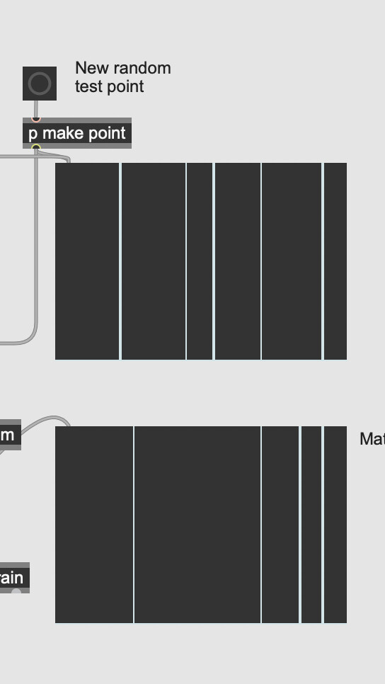
In the spirit of putting my rubbish where my mouth is, I’ve had a crack a the GMM idea with MuBu.
It doesn’t seem like the most efficient way of going about it, because you have to generate quite a lot of redundancy as far as I can see, by treating the frequencies of interest as 1s in a grid of 0s sampled-as finely as you want your model to discriminate. That said, it seems to do what it is I was imaging @a.harker might have been after.
----------begin_max5_patcher----------
3945.3oc6csziiaiD9bO+JDLBPtzQfuerW1rKvhbJ6kMXuDrngrMa2JirjWI
4Y5dB1+6aQRKaIqGV9U2FIdd31MIkHqOVUwpJRU52+zCSll8poXRveI3WCd3
ge+SO7fqHaAOr42eXxxnWmkDU3Z1jYYKWZRKm7nutRyqktx+kWLAIweNI17R
V17hfkwKdoLXpIXcg440IAOmkGTjszDjlUFmkFj8bv73hxnzYlfxrfR3xWFU
N6Ey7fUYwok+0pdHIN0LKacpqaXaJbksowoKdJ2LqzO7YLTH5Q3GX6Ovb2uI
fOC9Oatn34tQZ1ze6GvRY08Oc8x3zDSoi7v6JLacYUoHag+uO8I6GONRbZoo
nHZgoENAXjII1hQAnP3eH3OLt+688u8ZiVSXbRe0dvxufM3fWXsuHDJ4AaVe
8amijwO9OsKeu1bxnQm2vNYuwnA3uIRG+sVY+AQpcr4LZMFbOKa4aqL9KYxj
t484cx6S5j2GeB79vcXpIeR+zhR5IBDNjHIRL76RrlRzpGC7BtDxfz0iASlF
ktnG5itqqyiVZJM4OYRill3tbz3k6Im.s2m9wedixsx7n3T.M7Z4F.ivDjaB
mJEsAIrmYfzq5M70V815jx3hj346lmKh+lCfwDU+TkVK7DkrMQQPBOOM5Py8
cOuKzaGJ.kU9le9Fep7BvMAJEnZeG6XKw0FYmOuRp4qv.uEqxx0SWGB7Iy97
VtEXr3+9PBUDVHWiTZEUy3JlfK.0ERZHCowXLhiYJJlJsKNRGmL1.X8wr9Is
BQi9hY9Sv0Ci4mhJKyimttza9wCagnGl7ES9zrByVsOdX8Rs.7z0O+rIONct
40fuC+XvB.ZQGMrxH1B0DNAKDRlBwAXEqFAr1Mbptxpj6Ssz+z70f7nz4YKC
fYhxlZkZr1T0XYUto.tSQVq3dp6VzgxLX8+PJaOTDiYtEDQHJWJHRkP+Xfe8
MJsGMaBwUVyVeH0+FXZd9MvP0nx8ThW3sb0ZC6xBSxW.N5AscsW.b.qakZRn
pE9ArZbFmQoBFB3AQLRE90qguB9GD98ObZc8PEPaCHwAbBg7A4N5ccOA6Ch5
9EKGgyKle5m+4vf+UInkIn3kr0IyChVsxDkG.0OKKsHKwLr7Ua.gqc9zv4g7
8wiM94zu3B8CBP1.EAeMNIInHNAZSxaA4fufEdG9b.V7yVLK2DDWDjkBMHBZ
a5BfOw7ZzxUvOWYxCb81if6iA+1ZPG070qRhmAxOf.3x2BJdKEtGkwy7RiOB
NcNKx1KEyhMf6kch1hgL7R2VTiBFioPLFWnQBJhQU3sfuR1G3i9f.eSjUcTk
RJW6AmyAESVlvXPgU1WSC7KD9Hf6N9VuAGyhRR.qT+d2E+8gAt6jCWsSQQVi
69g4wKCxy9p0E9Hq7bd7qgAe078vz3BSpI2Oy.sz2yFXpyMuAy5SMVY.fGnl
FfFyKxAb.B6jBjnPIGovRXJRJkXNY6DArJSOyDb0GzLwO4ADiO1GUqzZA2EA
yiJiNVUAXNtMy4onXfKts8P.C57vJ3uHpTiHJJ47cPfy9igCBqxsxi9vkUbr
lt1oqWJbKKWa.bW6UQFjP+uqM4uM4HsMhfossPWvGlLIeLj4I5vmTHCYZsVp
EvPGLWRA91QDpqhCeL9stCeV3Dt8kYawrWh85SmLjwlHduFaRPsL1rWTy0UU
sJGzjO23POqg3aJc5hYYIY4aTjau0vRYJEgxseiIQbkpoFjDyhnYuYIrsWIt
FySsaGB7tBTS9XGeA2C2NicxgIKdQZF.gfUXe9vLAaYy2pD44rzxTnGck92x
iiRB96YIym7tMoyEL6jtf7mt4b567bN4lYNuSy5+yGG.R8NyAfuBb.8rNZYv
zfoCvBn6HFTZUnRxgRUfIlHBGbqiRN7hktceXvcgfcLgf+TLNroHPW1GP0ss
OvsiQZqABDgFrATSrFMvbTL6fTbmTJUeg1uE7kiUX82hstYbznCXbbKEBL4Q
xOruhgFfk3HhzK8cKt2mRPc619Sp7hFYbJ8JGY7CJFokiMzqmmXDQd6IFsB7
x7ylCtWkcCQbsSSChIHDDBKn.WmTdpLBjiwADb8wpIeeGNdNNw.NcT.b60Z8
CShVspVwOT6Rrv0u4W1cSrKrEEm1X4YqM.luDWc87skFkCHVI.Wqy8K+851.
UauMYyM4oqi24+ichayPxMEYW1rXUzL+EamIqptdPh8g.yyCpcFwvw0BMo0T
jjrYe1agBppvrUFvgy5J.ZT8byyQqSJext58t32D1Y8OuYD1YkMW5eKArHOd
dVpcPzXlvVbU2Yi5k+L8TmXbsHMZUGWr2gydpr.Hx0ESixsSTaDtHUUVlkkz
rpsWWh44xMUuJNMcOTrLaU+UlaOKT8W8zLnxkCcuc0T7z5TesOA7DkOYcttY
6hRR1HG271+ZTZ7xnRSYreJ.jFqpzqf4khY4YIIMnWeMeoiZlC73yLeMdd4K
tNpNy.z73UULQS1NKOOdgonrYYkQKJZVx1PxUqn0S2HC+ToY4pDfJZ1.P5Ht
nr3kruVrogULZ0Afcmws5xz0UJ1n7gTN1TA42RBV.18updkcpfLDVrfSnHkf
yjJaPqoZXIDrBKIfE6XLmh0VI180ONhfb1RWIlWe7z0Bm8YC5tnu7P0xGmBh
0zHjtcHnWG0vXqy4Ta.r0fc4XMiJQf0p1iHh1V0Hfm9gF1I.M32InAcHngoB
I1f2Z+.izZ0UDnHev.0vRcEVPYbLRXQnjJ.C5Ud4LtzskIx8AxyVpC8AK0M.
hYcMN4.3kh53Y.+hzNSaId3RC1xAUcBvUkyP8CYHcuPF9iFxZ5B4A.MoJjZ0
vi3dPSJ6xuwi22w9ieywvjQe2DKGyhgafLDJjKrxkZOjY8d7xr7GhcSKHdP0
VN9FL3GoTgUDL0iOBkGYFMKU+3C+Dj5dmTsuYKxOrfWELIngXqlIkXijG.SR
53fogkzD2tK.Z0MwO..s4voHBo1v8wPaV7S6J6JnXR9AqXx0eiBSX9ygORH2
fI1y2i6zRfNOAKR+1Lg5mkoVMUGij5t335DaX6tz7W9wvI34BihCsA1Qp2.f
8heM.G5In0Actfyt.FXCqYOtA5naa8ciZEYqymUwAr0AqfljJ36aYb51.n7q
0nZaKG071QONrLbiabXEOudiCqUIA3wLNpPtqy3v5c23viq73fbiLNPidbvt
5iiwwePt57ojQMNPW0wgdz3wFj6JNNFm9C0UEOFsba0H9JMNjicdAwt5iiQw
mhtp5OPidcNq0xWwwgXzii1bRKim6eNMpNHHB2I9RSBAep.Grnrs9Woo9ydZ
qp5jv1TX0l0L1i61QEk7EIYSiR1Kz1cED8S+fycl68WGGpBvZwPtMXQTBRJU
1CN+Ys0er6a828s969V+ceq+tu0e225u6a828s969V+ceq+tu0e225u6a828
s969V+ceq+tu0e225u2os961LTj+QJVu2Jw99VYu.tU1ajak8J5VYuytQ1Kw
ak8V8lYuluU168ajyhvsxYy3V4rpbQN6N+wdq+J2FvnwtieT6S.Xq7ik9D2w
O8wjtlvWT593obBGbyBnesyqBk15SQ6XvdD4oHs7J+ji2a11wrxjNOnVlnwk
65Rmera+qTFBEf.CVQ.tPYJWBohbpbChqL2PeOxzXLdnGfbIZjYWoQkRi6hx
knq7C+beT970KWMTRyg5BuNAHr8yQWzSUlmKu1Yk5gxwTKVtbHlbreeVZoxy
87Mi0RvCYJ09HfKHCkgo37OnrN+pjn2B9N7HxCRmZBPny4T109g2uLawhc4S
yAHKFuiD8xHdb86KONvvefOr98MKenDFFWnZyFaS2d6iLzSUU8tTAx6qPrKC
pAxvsyeZA+3hn0EEwQoEA7feL2rXcRTd72bF6E.5ur++XwLXEuPqdOglPEXE
EKjPgB7Qjj0FJYqQOF0D7KuA.0RUHCfLDgniztWWm7KLlep7SzOnk9mkXhxe
LHZ9bu0P3fezZAdEOkOqmNKKovkLKCruwCbfVQ8rNyXStyTar9D.6DSyXBlR
xnVMw5Pr.yYbJRQTDtKu+CpyrlW.K1vzfklZL0ulywhqnO7rpRG1MJPmlR5d
yoJD5sWJUwtc7wGIv.pX5fWPMBmLNX9Hh8w3qgUgcck0GIfv3L21PnwfHfhx
QDalO+jOfozS37kNRO9MKmt2Y5Cf.q67I1ShZis.YHlz5UtDbJqU04lBWByd
6ccaM1A5B+QLcWYoQqx2bf5vHTsyw2kIWbdxYkqN49o71o74KZR4hbh4jK2M
q4tK4Qm8CJ0FLpUvnnMhEUewgx9B6oJN1slHFaW4ds3b39h2HJcSxxm6OC0n
2iNmR6tywmWmyFEJyaDu182pNoTDp2OYmQAImVIaWMXbHAVcFXhQRv+C2p4i
ukXknkS0fHp2MlV0cwmnDxwfUhZ6zzI2WNle5A6J0Uggbuaaect7BPmtTW1A
6q8TErG6mVQ5HziXk675QA+ProbOFG3Q3RYGgkpcKu3RYjQw4P3uaH59RzWJ
VG14Oc1o1DhVOxoyNZ4kd5bbBm7qiBaaRxb2Vq9NuTEcTKUwtH7w1vHsau45
iUBMDqjM2Z1Q5oTYe.CXRIRCKqP3bl8rOQB4sbyrcKOShhLN7CewvuCqy4Rs
XE6.8D+hvTP0ixVIwEouFkj10xtrQM4wtHKXLl9RKdurpQ13LarCPImWWqO6
El5d4FPGg0aaPKgVnQbPewiitkmIbxnmMMI1D9Qg1ZB9Xnh1s7LoBt77oB+K
1X6i24Hoh1s7LoB8nrYldADhziAuzpKUOgeW5IwXnoKgCGiZUQ1kXdZb1JQG
hulH6J9dnMYodNUgsrvXoO32pQzxy1nhwXSF8hrpzXV78Rr92dlPdJyScZ8H
i.Jknbv8RFGYeSVf6aZpUCaPQ9.os2yfukX16Yueum691Oy88+71u+yZu6na
4eti2K3caOpUKidUr8Itu5IZuIR29s6wtOPg67Ja6KtimhSszno16LrceT+k
1QzrYlzlurOT1lAnJAKbuEQPZEhs4p9ztSilMTwvkt+iTs+MxVkCR04hZPv0
dVJ5ljaLjXDJmncu2QjDNy8MhjYeMZbYGVM1nttGXGOFOcwywIIaIn5wsuJL
xSVjGMOd2q1uMzOd6bh.9i7wN+FtdRKvcYjpKa2a.l1eq8kUcU1GKSsatmtY
t29MnH7dWUj8cnoyfRYsX6uJOaUV9177PHUus8qKy1RnUtPuMz+cO80T5Xby
h0etSFA2kaNiwqd01v.ZlpOYNKuRldxpFe5+8o+O.hdm7
-----------end_max5_patcher-----------
This way queries are visualised are pretty cool:
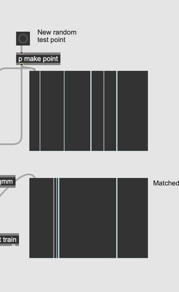
Sometimes I get something like parts of the data are shifted:
but overall the matching actually seems pretty clever in capturing the distribution. Thanks science
That is roughtly what I was hoping for from the normalised bandpassed bands I described above, and was hoping an autoencoder would remove the bands that are always small. Was I too hopeful and deluded? I will try it with your patch anyway later this week once I’m done with all the videos/presentations I have to do…