FluCoMa vs Librosa (NMF)

I’m trying to figure out why I get very consistently different results when doing NMF with Librosa vs with FluCoMa. I bet someone here knows the answer. @weefuzzy ? @tremblap ? @jamesbradbury

I’m trying to be as similar as possible in the execution but continuously get these different results (code below). This is the first three seconds of the FluCoMa test soundfile “Tremblay-BaB-SoundscapeGolcarWithDog.wav”.

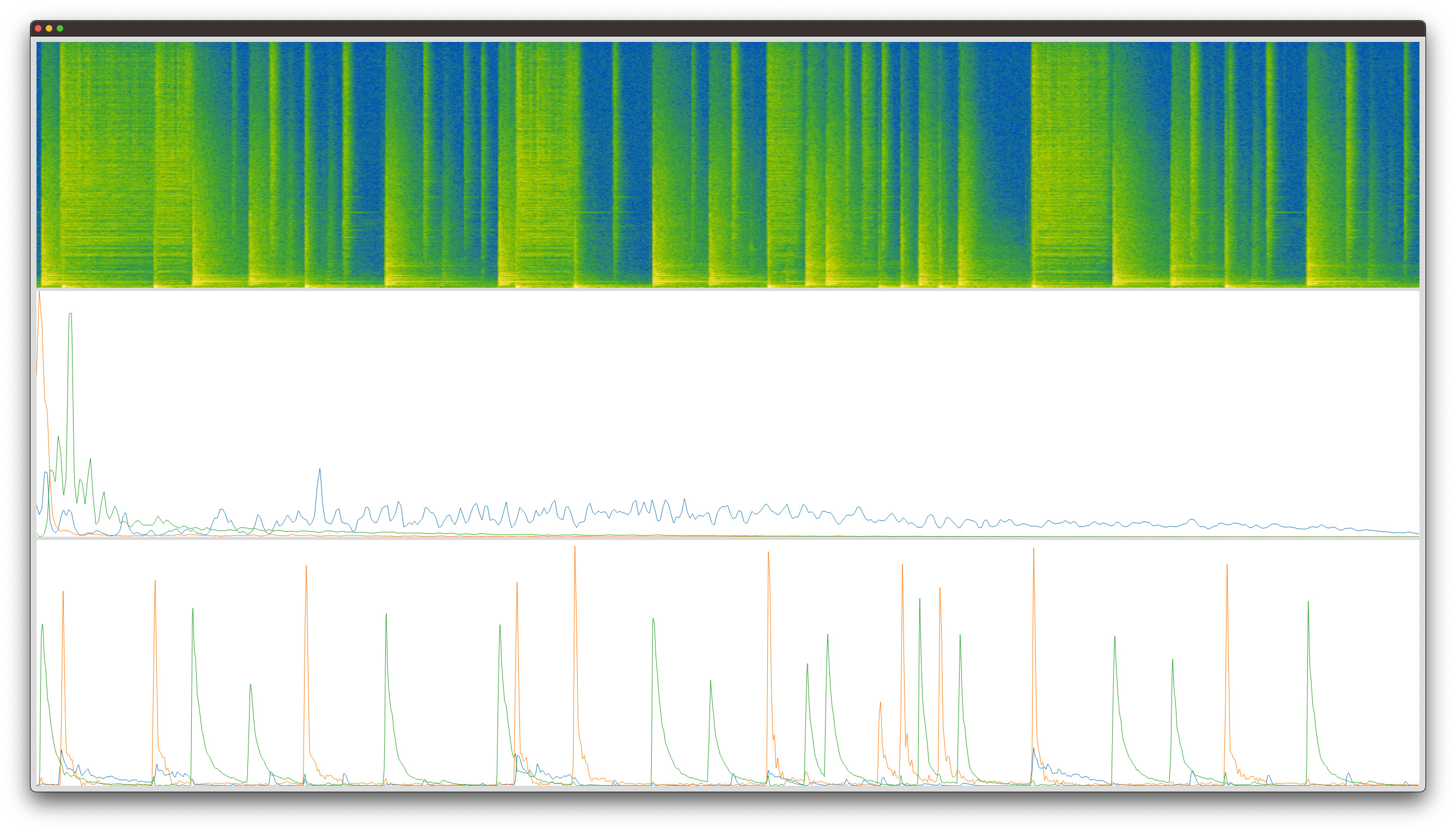
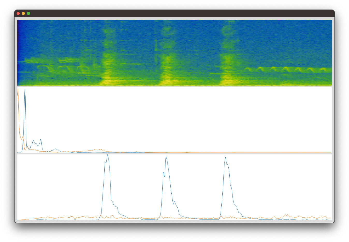
FluCoMa (spectrogram, bases, activations):

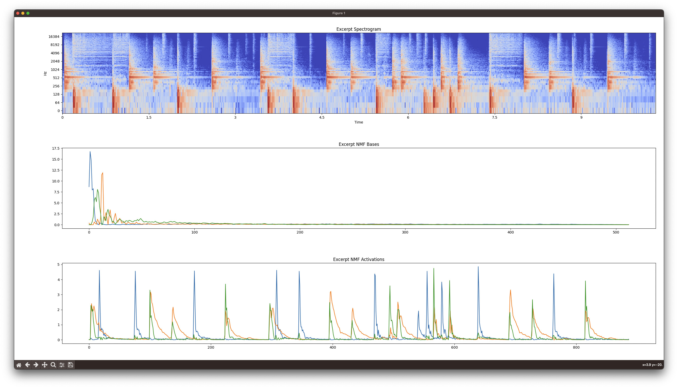
Librosa (spectrogram (log by default), bases, activations):

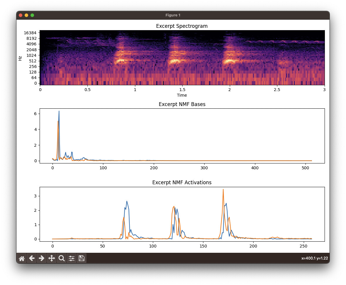
You can see that FluCoMa consistently separates out the dog bark (blue basis and activation) from the “other” in the sound file. Librosa does not.

Audio Results:

I’ve also resynthesized the buffer in Librosa and FluCoMa to aurally compare:

https://drive.google.com/drive/folders/1cx8wDh9DNhH2GoIpsbpaJzPtOg5PY7X0?usp=sharing

It’s obvious to me that FluCoMa works better (sounds better, separates better). Why is this? How could I get as good of results in Librosa or Python generally?

Code:

FluCoMa:

(
~thisFolder = thisProcess.nowExecutingPath.dirname;
fork{
	b = Buffer.read(s,FluidFilesPath("Tremblay-BaB-SoundscapeGolcarWithDog.wav"),numFrames:44100*3);
	~bases = Buffer(s);
	~acts = Buffer(s);
	~src = Buffer(s);
	~resynth = Buffer(s);
	s.sync;
	2.do{
		arg i;
		FluidBufCompose.processBlocking(s,b,startChan:i,numChans:1,gain:0.5,destGain:1,destination:~src);
	};

	FluidBufNMF.processBlocking(s,~src,bases:~bases,resynth:~resynth,resynthMode:1,activations:~acts,components:2);
	~mags = Buffer(s);
	FluidBufSTFT.processBlocking(s,~src,magnitude:~mags,action:{"done".postln;});

	~tmpBuf = Buffer(s);
	2.do{
		arg i;
		FluidBufCompose.processBlocking(s,~resynth,startChan:i,numChans:1,destination:~tmpBuf);
		s.sync;
		~tmpBuf.write(~thisFolder+/+"flucoma-component-%.wav".format(i),"wav");
		s.sync;
	};
}
)

(
~win = Window();
~win.layout = VLayout(
	FluidWaveform(imageBuffer:~mags,parent:~win,standalone:false,imageColorScheme:1,imageColorScaling:1),
	FluidWaveform(featuresBuffer:~bases,parent:~win,standalone:false,normalizeFeaturesIndependently:false),
	FluidWaveform(featuresBuffer:~acts,parent:~win,standalone:false,normalizeFeaturesIndependently:false)
);
~win.front;
)

Librosa:

import librosa
import librosa.display
import numpy as np
import matplotlib.pyplot as plt
import soundfile as sf

def resynthComponent(stft,basis,activation,outpath,fftSettings):
    Y = np.outer(basis, activation) * np.exp(1j * np.angle(stft))
    y = librosa.istft(Y,**fftSettings)
    sf.write(outpath,y,sr,subtype='PCM_24')

# Replace 'your_audio_file.wav' with the path to your audio file
audio_file_path = '../audio-files/Tremblay-BaB-SoundscapeGolcarWithDog.wav' 
n_components = 2
sr = 44100
fftSettings = {'n_fft':1024,'hop_length':512}

excerpt, sr = librosa.load(audio_file_path,sr=sr,duration=3,mono=True)
y, sr = librosa.load(audio_file_path,sr=sr)

print(audio_file_path,sr)

excerpt_stft = librosa.stft(excerpt,**fftSettings)

print(f'stft shape: {excerpt_stft.shape[0]} mags, {excerpt_stft.shape[1]} frames')

bases, activations = librosa.decompose.decompose(np.abs(excerpt_stft), n_components=n_components)
bases = np.transpose(bases)

print(f'bases shape: {bases.shape}')
print(f'activations shape: {activations.shape}')

for i in range(n_components):
    resynthComponent(excerpt_stft,bases[i],activations[i],f'librosa-component-{i}.wav',fftSettings)

plt.figure(figsize=(12, 8))

plt.subplot(3, 1, 1)
librosa.display.specshow(librosa.amplitude_to_db(np.abs(excerpt_stft)), sr=sr, x_axis='time', y_axis='log')
plt.title('Excerpt Spectrogram')

plt.subplot(3, 1, 2)
for basis in bases:
    plt.plot(basis)
plt.title('Excerpt NMF Bases')

plt.subplot(3, 1, 3)
for activation in activations:
    plt.plot(activation)
plt.title('Excerpt NMF Activations')

plt.tight_layout()
plt.show()
1 Like

Just to verify I get the same results. I tried a different sound file and in that case the outputs were the same. Is it like this with everything for you?

Also -

1 Like

Also - !?

Just to be clear, are you saying saying (1) you got the same results as me for the Golcar file, and (2) you tried a different sound file and your Librosa and FluCoMa outputs were the same? So it didn’t work like mine in (1) but your Librosa and FluCoMa seemed to match in (2)?

I first noticed this when I was testing with the “Nicol-LoopE-M.wav”. Nicol makes sense to use 3 components… so I though I would try to simplify things to a file that I know has consistent success (in FluCoMa) with 2 components: the Golcar file.

Nicol-LoopE-M.wav:


https://drive.google.com/drive/folders/19SaSqrcHPGI9F-L4N9qQX0E6Oe84ICSx?usp=sharing

The results in the images above are very consistent for me (of course there’s some variation due to the stochastic nature of the algorithm)! Notice how in Librosa, the green and orange activations are pretty much always together in time.

A few thoughts:

  1. Could the padding strategy be different?
  2. Is FluCoMa scaling (non-linearly) the magnitudes of the STFT before they get passed to NMF?
  3. This might only relate to the resynthesis, but, Librosa (the Python code actually) is using the phases from the original file to resynthesize. Is FluCoMa doing that or something else?
  4. Is FluCoMa adjusting the magnitudes such that the output component buffers will null-sum? Or perhaps that an HPSS-like masking going on to manage the balance between matrices? I don’t think that should matter for the NMF algorithm, as I think it would just be on the output, but *shrug*?

I poked at the C++ a bit to try to answer these questions, but unfortunately it is a bit opaque.

Hi @tedmoore

From a very quick glance (bleary, still on coffee #1) librosa is using sklearn to do the NMF. If it’s just using default settings for the sklearn object, then it’s not surprising that things sound different. I’d suggest comparing against sklearn directly until you’ve pinned down what’s up.

Two sklearn parameter defaults that are definitely different to flucoma are:

  • solver: we use multiplicative updates not coordinate descent
  • beta_loss: we use ‘kullback-leibler’; if librosa is still using the default ‘frobenius’ then this could make quite a bit of difference

As for your questions above:

  1. The padding strategy could be different, but I wouldn’t expect it to account for all the differences you’ve encountered
  2. Don’t think so – think we just use the magnitude spectrogram
  3. Flucoma is using the original phase in resynthesis, yes
  4. Don’t quite follow, but I think the answer is ‘HPSS-like masking’
1 Like

Thank you @weefuzzy ! These are excellent things for me to pursue. I’ll do some investigating and report back.

So strange. I responded to this but don’t see my response here.

With 16 bit files, the two softwares get the same results. With 24 bit files they get different results. Not sure if that helps your sleuthing.

Sam

1 Like

:eyes: Very interesting. That is not something that would have been high on my list of considerations. Might be worth fiddling around with the numpy data types to see if that helps get a grasp on it too.

Thank you again @weefuzzy, I figured it out!

It was this:

I’m now using 'solver'='mu' and 'beta_loss'='kullback-leibler'. It now matches FluCoMa’s decomposition. The resynthesis still doesn’t sound as good… perhaps there’s more investigating to happen there.

The code is a bit more noodly now, but there’s a script for decomposition, resynthesis, and seeding. For what it’s worth, sklearn’s NMF doesn’t allow for a FluCoMa-style basesmode=2 or actmode=2 where the bases or activations respectively don’t get updated at all. But one can seed a la bases/actmode 1. I think that when one seeds the sklearn one, both bases and activations need to be provided, so I’ve been manually creating a random initialization for the not-seeded part.

My next question

is how might one implement a FluidNMFMatch kind of thing in Python for non-realtime (obviously) processing. I think the goal here is to retrieve bases of a known sound with a small decomposition (short sound file) and then use that to create activations from a much longer sound. I’m thinking this will be good so that one doesn’t need to try to do a whole decomposition of a massive matrix that would take a week to compute.

I’m thinking that in order to imitate FluidNMFMatch I would get my bases that I want to seed and then loop over every FFT frame in a matrix of magnitudes and do a NMF with the bases seeded. Each FFT frame would create new activation values for that FFT and if I collect all of these and put them in the right order, I’d get the activation curve (or ‘match values’ or whatever we want to call them) that would come out of FluidNMFMatch.

This strategy of many bases-seeded small NMF computations should be much faster than trying to compute the decomposition of the hole matrix. I tried this but the resulting “activation curve” was just noise… quite possibly because the NMF decomposition done on each FFT frame’s magnitudes was “seeded” with the bases, but then randomness for the activation…?

Any thoughts are appreciated!

That’s pretty much what NMFMatch does, yes. Now, answering on low caffeine again, but casting my eyes over the sklearn docs and source:

  • Looks like they swap the meanings of W and H from what’s conventional so that W is the activations and H is the bases? eeek
  • It doesn’t look like you’ll ever get any love from sklearn.decomposition.NMF for this, because it gives you no choice about updating both matrices. So, yes, garbage will ensue: you’re just doing a refitting on a really small input sample.
  • However sklearn.decomposition.MiniBatchNMF might be useable – it has an internal _fit_transform method that allows you to switch off updating for the bases (if I understand their naming properly).
1 Like

Thank you @weefuzzy! This feels promising. I’ll report back when I do some testing!

Thanks again @weefuzzy, your suggestion was right on the money.

The _fit_transform method that has the optional update_H=False flag is actually part of the NMF class, not MiniBatchNMF.

“FluidNMFMatch” “in Python” works:

I tested my new nmf_match.py on “Tremblay-BaB-SoundscapeGolcarWithDog.wav” by:

  1. Decomposing just the first three seconds of the file (using nmf_decomposition.py) to get some bases (one of which will represent the dog bark)

  2. Pass those bases and the original file to my nmf_match.py. It looked exactly as I would have expected.

double check

Just to make sure that the Python code wasn’t just, somehow, actually just re-doing decomposition on the whole matrix, I repeated steps 1 and 2 above with a 2-hour audio file. Of course the decomposition on just the first 10 seconds (yes, I did 10 seconds the second time, not 3) was quite fast and then when I passed those bases and the whole 2-hours to nmf_match.py it chewed through the whole thing in 2 minutes (so obviously it’s not trying to decompose the whole 2 hours).

The results were not really intelligible, mostly because I don’t really know what is in that 2 hour file, but it felt important to test.

1 Like

that’s cool, because you could tweak by ear in Max/SC/Pd the nmf parameters and even the bases, and then when you are happy, you can run this in NRT in python!

this opens up cool workflows, thanks for sharing!

1 Like