Class "interpolation" (distance to classes)

[rodrigo.constanzo]

Revisited this idea today based on @weefuzzy’s awesome outlier rejection stuff from this thread.

So as a reminder, the general idea is that (based on a great suggestion/chat with @balintlaczko) each class would be one-hot encoded and then fed into fluid.knnregressor~ where the amount of nearest neighbours would be be used to determine how much of that class it was. If all the neighbors were the first class, that meant it was 100% that class, if it was 50/50, that would be 50% etc…

My thinking/hope was that using outlier rejection to create a more condensed and representative “class” would therefore make the one-hot encoding more accurate, therefore when moving from one class to the other, that that would create a smoother overall change.

I put that hypothesis to the test today.

////////////////////////////////////////////////////////////////////////////////////////////////////////////////////////////////////////

So firstly, given @weefuzzy’s suggestion here:

@weefuzzy

As a rule I’d say pre-, especially if the DR is just being used for visualisation and the actual classification will be done in higher dimensions.

That I’d compare the 104d space with outlier rejection with the best results I got before (31d PCA of 104d, created by keeping 95% variance).

By going with moderate outlier rejection settings I kept about 80% of the entries.

That gave me results like this:

(umap project is almost identical in both)

Here’s a close up of the interpolation plot:

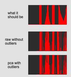
As a reminder, the top one is a platonic version of what I’m doing on the drum. Some hits at the center, some hits at the edge, then slowly moving from center to edge, then doing the reverse again.

The whole pattern being:
*center / edge / center → edge → center || edge / center / edge → center → edge

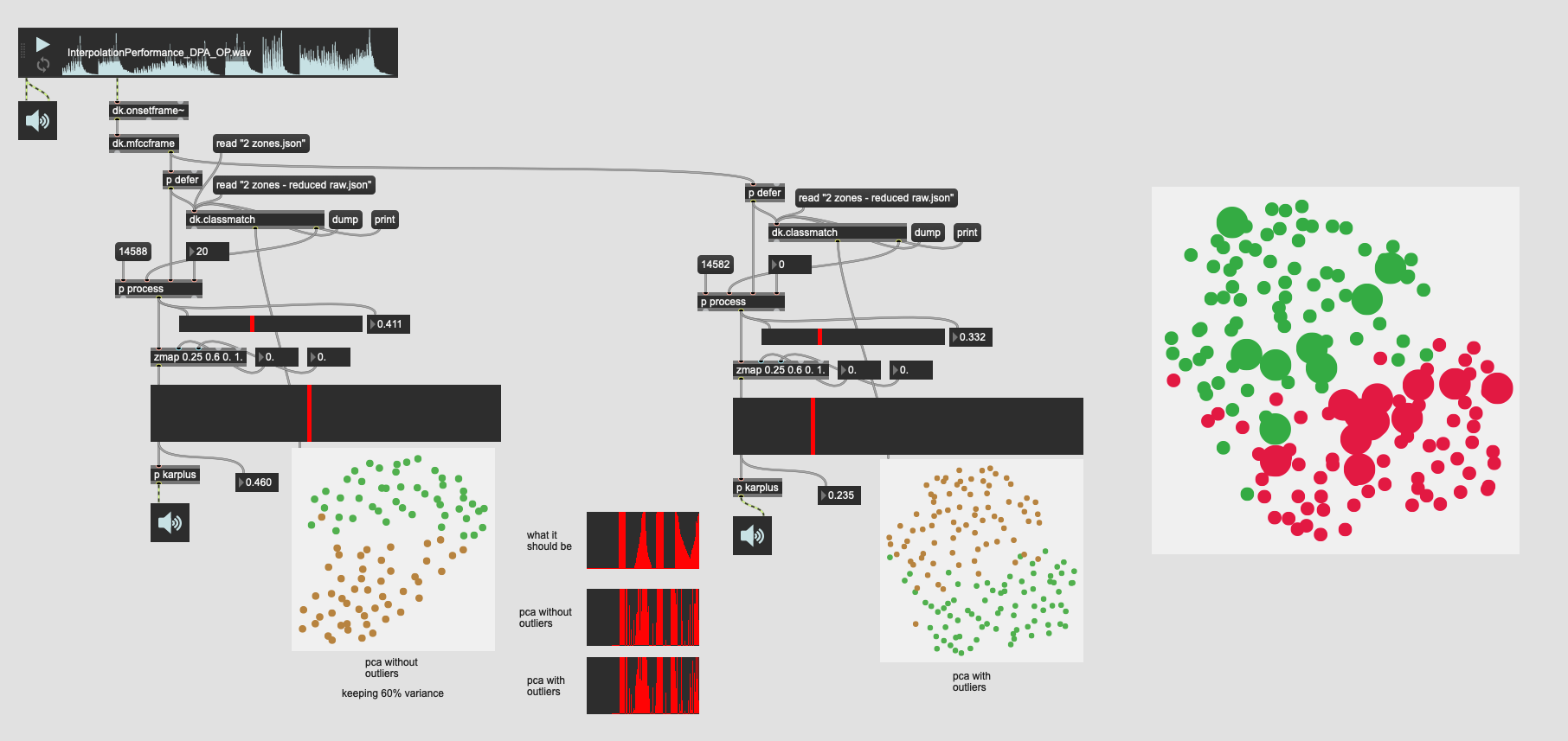
Here’s what it looks/sounds like:

104d with outlier rejection vs 31d PCA with all entries

(the main thing to look it are the big sliders on the left and right, as well as the one-hot encoding on the right showing how the nearest neighbours (40 in this case) are “interpolating”).

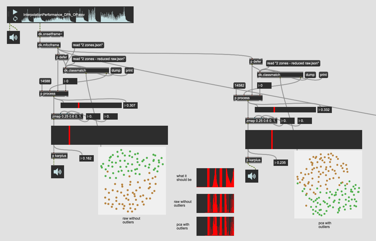
So the initial jumping off point gives me… nearly identical results to what I had before. I figure, ok, that’s a good place to start as this is operating on the full 104d, which wasn’t as good as before.

////////////////////////////////////////////////////////////////////////////////////////////////////////////////////////////////////////

So let me try to improve it by going with the PCA and outlier rejection. Surely that will make a lean and mean classifier!

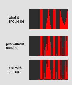
So this is 31d of PCA’d MFCC (keeping 95% variance) then running that into a more aggressive outlier rejection where I keep ~60% of the entries. And comparing that to the 31d PCA with no outlier rejection.

Here’s the results of that:

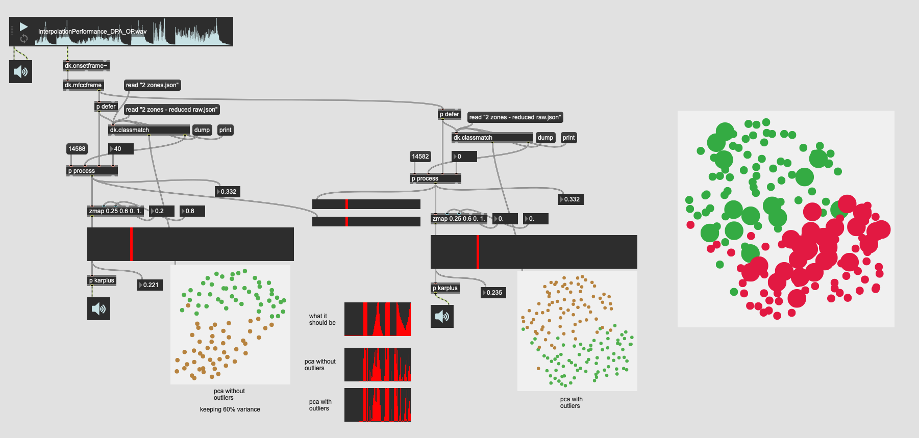
You can see that even though there are significantly less entries in the plotter that the separation between the classes is still quite good.

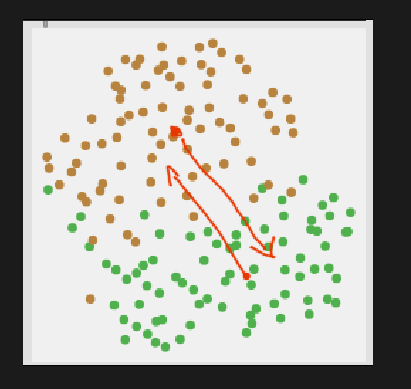
And the closeup of the trajectory:

It’s near identical!

In this one I’ve actually adjusted the scale object range to have a slightly better “dynamic range”. If that wasn’t the case, the plots (and sounding results) are literally identical.

I double-triple checked this thinking I did something wrong somewhere…

Here’s the sound/look of that:

31d PCA with 60% outlier rejection vs 13d PCA with no outlier rejection

////////////////////////////////////////////////////////////////////////////////////////////////////////////////////////////////////////

Finally, as a sanity check I tried the same but with fewer neighbours in the kdtree to see if that helps make things smoother.

So data/processing wise this is the same as the version just above it. 31d of PCA’d MFCC (keeping 95% variance) then aggressive outlier rejection keeping the inner 60% of entries.

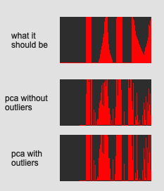
The overall plot looks the same:

The trajectory is a bit varied, but very very similar:

And here’s the sound/look of it:

31d PCA with 60% outlier rejection (20 nearest neighbors) vs 13d PCA with no outlier rejection

So like the others, not very much difference.

////////////////////////////////////////////////////////////////////////////////////////////////////////////////////////////////////////

So my main couple of takeaways are:

1. It appears that there is a limit to how smooth this approach can get with one-hot encoded nearest neighbours. Since the classification tends to be fairly binary where it kind of “flops” from one class to the other means that the “interpolation” being shown here is more accidental than what can be extracted.*
2. It is absolutely brutal to take apart and process datasets/labelsets. I had kind of overlooked that you can’t use fluid.datasetquery~ on labelsets, which made for a lot more manual packing/unpacking than I was thinking.**

*I still think this is a useful approach, and I’ll include as a refined a version of this as I can get in SP-Tools (unless I figure out something better, more on this below).

It’s not as smooth as I would like, but when working with only classes as a jumping off point, it’s at least “something”, and if being used for something more interesting than walking up/down a melody, can hopefully add a bit of nuance to some mapping.

**In terms of processing datasets. I do feel like some way to split/iterate/pack datasets (and labelsets) would be very helpful. I thought I had already baked some code to do this, but it turns out it wasn’t generic enough, so in order to do all the stuff above, I had like 4 patches open, and was dump-ing little bits here and there manually just to test the results. Really really tedious stuff!

////////////////////////////////////////////////////////////////////////////////////////////////////////////////////////////////////////

NOW onto this:

@weefuzzy

• Does an [cool outlier rejection] have any useful implications for computing class “interpolation”?

Don’t know. Will need to remind myself of what you’re trying to do there and think more about it. But just have a play in the meantime and come back with Qs.

So after processing how useful outlier rejection would be for general classification purposes, I thought that since the algorithm used (local outlier probabilities) returns back a 0. to 1. for each point, and that it’s possible to

@weefuzzy

test new incoming datapoints for outlier-ness in terms of the original fitted data

that this may prove useful for interpolation.

One of my earlier tests in this thread was to use class means, and specifically, distance to class means as a way to deal with “interpolation”. That failed, I think, because MFCCs are quite ornery and the mean of a bunch of MFCCs/stats does not represent a useful point of comparison to. And being that MFCCs are intrinsically bipolar, that it just makes for a statistical mush.

Now with this LoOP approach, there’s a more meaningfully computed measure of how far from the central cluster something is.

Now I’m thinking/typing out loud here, as I don’t fully understand if this is possible with the current algorithm. But what I’m thinking is that each class is run through the algorithm to create an outlier probability, and that new incoming points would be tested against both of these probabilities. Then the relationship between the two outlier-ness values (one for each class) would signify whether it is more one class or the other. Something like this:

Superficially that makes a lot of sense to me, but it gets fuzzier when I think about how to determine directionality here, like what if I start dead center in one class, and very distant from the other, but then I start moving “away” from both classes:

So there’s an aspect of that where this gets confusing.

////////////////////////////////////////////////////////////////////////////////////////////////////////////////////////////////////////

SO

This last chunk is more a follow up question for @weefuzzy based on the outlier rejection stuff from the other thread.

Is there a way to implement the outlier rejection such that once computed/fitted, a new incoming data point can be checked against both classes in a way that would offer a smooth(er than I get with one-hot encoding) “interpolation” of where you are relative to both classes?