you know that this is exactly what the mlpclassifier is doing, and that I shared a patch doing this and sharing it here in April 2022 and pointed at it in May last year? So I wonder what is different now?
thanks for sharing - you are in good company with @balintlaczko here. I look forward to see how (short) time series will work (with lstm) but in the meantime I wonder if you could not bake in some sort of spectral profile à la LPT instead of averaging… the sound you compare have clear spectromorphologies after all, and you dismiss the morpho part ![]()
I remember looking at this back then and although I don’t remember the specifics, I remember not finding it useful for what I was doing.
So I loaded it up into the current patch with the current sounds encoded just as it was in your patch, using a dataset/labelset (as opposed to the mlp example above that is dataset/dataset so it has the “one-hot” vectors). And I get this:

(in effect, the mlp-based stuff doesn’t seem to be able to actually communicate confidence (other than flip-flopping between 100% this or 100% that))
When I did a ton of testing with this stuff in the past (LTEp) I found that this worked well for having a visual representation/spread for something where you mouse/browse around ala CataRT, but found that it didn’t work with classification nearly as well. I never tried using just purely spectral moments this, so that’s my next course of action.
My thinking, though, is that the “one-hot” approach is only as good as the core classification that can happen with it. e.g. if I don’t get good solid separation between the classes with the descriptors/recipe, it likely won’t work well for this at all.
So there’s some refinement here still I think(/hope) in terms of optimizing the descriptor recipe, but also curious if there’s anything else that can be done with regards to how interpolation/confidence is computed here. (e.g. mlp not working well and flip-flopping, numneighbours being one of the biggest deciding factors, etc…).
I do look forward to experimenting with this as in my case I just have 7 frames of analysis anyways, so I imagine I could just chuck all 7 frames in, rather than doing statistics on them and this would only slightly increase my dimension count while at the same time better representing morphology.
1 Like
Ok here is some further testing this morning.
I’ve wanted to visualize the numneighbours and see if a radius was useful at all, so I set up a fluid.kdtree~ trained on the same dataset to try and visualize things.
I don’t know if this is a useful/direct analog to fluid.knnregressor~ trained on the same input data (with “one-hot” vectors as output). As in, are the @numneighbours in fluid.knnregressor~ doing (mathematically) the same thing as @numneighbours in fluid.kdtree~?
Either way, here’s the same chunk of audio as in the previous examples with a few different settings:

I talk through it in the video but my first setup is @numneighbours 40 @radius 0, which more closely matches the settings in many of the examples above. Again, don’t know if this is mathematically the same, but kind of interesting to see that it jumps around a bit at the edges rather than being completely blobbed on one side.
Then I tried @numneighbours 0 @radius 50 to rely solely on radius. Not as good as results as I would have thought, particularly since I have to crank the radius up otherwise it misses some hits completely.
Finally I tried a hybrid, @numneighbours 10 @radius 60 which actually looks very promising. The center and edge classes seem decently defined and the interpolation looks a big more legible. Probably some fine tuning of the parameters here may be useful to tighten things up, but it’s definitely seems like an improvement.
////////////////////////////////////////////////////////////
And chasing up on a hunch, here is the same test but with the 31d PCA reduction (un-normalized) instead of the full 104d MFCC soup:

I tweaked the numbers slightly so they are comparable to the previous test:
-@numneighbours 30 @radius 0
-@numneighbours 0 @radius 50
-@numneighbours 10 @radius 70
To my eyes this looks quite a bit better actually. This leads me to believe that in this specific context it may be beneficial to do the PCA reduction.
THAT IS
If the maths are the same for @numneighbours in fluid.kdtree~/fluid.knnregressor~.
////////////////////////////////////////////////////////////
So with that being said, firstly, are the maths the same in these? And secondly, is there a way to somehow combine these to be able to use radius+numneighbors in a “one-hot” vectors context?
it is exactly the same code - it is calling the same kdtree code as an instance of that object. The beauty of C++ when well done
1 Like
Interesting!
Ok, so is there an elegant way to do what I’m doing above in reality? (as in, the moving slider and sonic results in the videos above are just the fluid.knnregressor~ in the background like in all the previous examples)
What comes to mind seems really clunky:
-getting the knearest numneighbours as a long list
-iterating through that to getpoint a parallel fluid.dataset~ with the “one-hot” vectors for each individual match from the knearest list
-manually do the maths to turn the “one-hot” vectors into an interpolated result (just averaging the values? eucledian funny business?)
-turn the results of that math into a single vector that represents the interpolation
And all of this would need to happen per hit and it feels like iterating/uzi-ing through lists and datasets would be kind of slow in this context.
Is there a shorter and/or more elegant way to do something like this? (is there a technical reason why fluid.knnregressor~ doesn’t have radius in addition to numneighbours if it’s doing the same kind of thing under the hood?)
Ok made some time today to dig into this today and some interesting/promsing results.
//////////////////////////////////////////////////////////
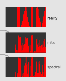
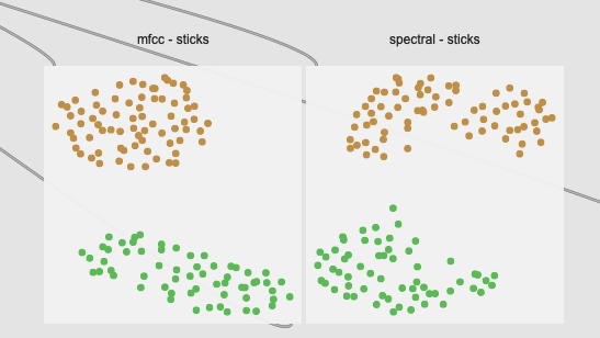
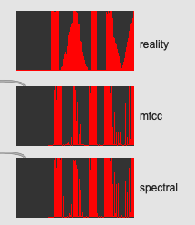
First some plots/comparisons.
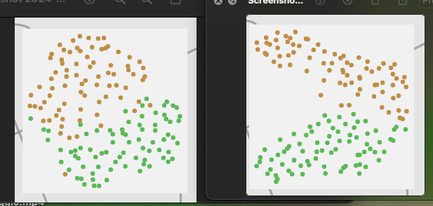
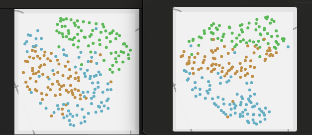
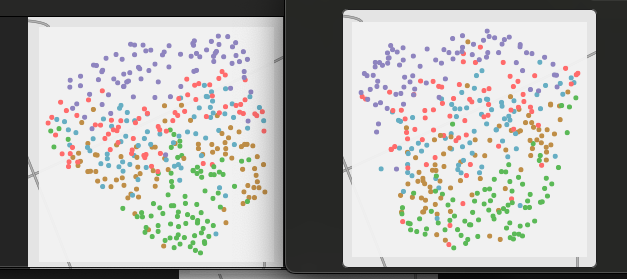
On the left are 2d UMAP reductions of 104d MFCCs and on the right is 2d UMAP reduction 56d spectral descriptors (all 7 spectral moments, min/mean/max/std, 1deriv).
2 classes:
3 classes:
5 classes:
8 classes:
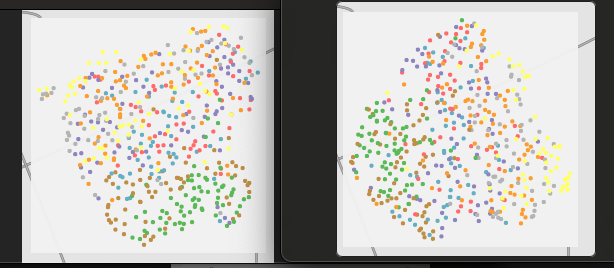
Overall the spectral moments look a bit more tight/tidy I have to say. It’s pretty close overall though, with the most clear difference being in the 3 class version where it’s closer to 3 clear stripes rather than a fuzzier middle area.
//////////////////////////////////////////////////////////
The combined vector confirms this. Here’s a vid showing the 2 class comparison. (we’re listening to the spectral moments being sonified):
 vs Spectral Moments (56d)")
The spectral moments seem to use the overall range better (no scaling being used here), which is perhaps indicative of a more clearly defined egde cases across fewer dimensions. It also looks to be slightly less jumpy overally, and specifically in the transitions.
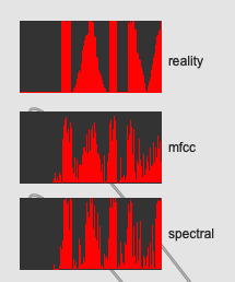
Here’s a multislider showing the plot over time:
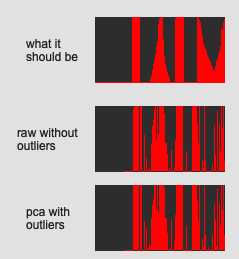
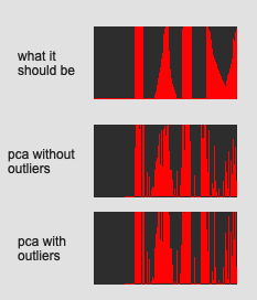
The top is my attempt at hand drawing what the output should be:
center / edge / center → edge → center / edge / center / edge / edge → center → edge
The “dynamic range” of the spectral moments stands out here, and you can see it is much less jump in the center → edge transition (less apparent in (edge → center however).
I don’t know if this is a useful metric for superficially checking the salience of data, but when keeping 95% of the variance with PCA, the 104d MFCCs becomes 31d PCA (~30%) and 56d spectral becomes 12d PCA (~21%), which would lead me to believe that the spectral moments are more redundant, but not sure.
//////////////////////////////////////////////////////////
Here is the same being plotted with fluid.kdtree~ so we can visualize the neighbors/radius stuff.

As before, I tweaked the numbers slightly to be more in line with previous ones.
-@numneighbours 30 @radius 0
-@numneighbours 0 @radius 24
-@numneighbours 10 @radius 24
The radius is perhaps too tight here as in some of the transition hits you can see the @numneighbours disappear completely.
Again, this looks slightly better than the 104d MFCC and 31d PCA’d MFCCs above. I will next try this with other source material (different drum classes, voice, etc…) to see how generalizable the 56d spectral moments are, but so far this is looking the most effective.
I also plan on experimenting a bit with different spectral statistics (min/mean/max/std at the moment) and/or perhaps leaving out derivatives at this point.
//////////////////////////////////////////////////////////
At this point I think I’m also just focussing on making it work solely with 2 classes trained, as even though you do get a bit of improvement in some cases from interim classes, this becomes a lot more practically and conceptually faffier (e.g. not being able to use pre-trained classes as they are, and having to manage tags for “real” classes vs “interpolation” classes etc…).
Aaand a bit of classic number crunching.
Compared the MFCC and Spectral descriptors in terms of raw/straight classification (ala all the experiments from this thread) and got the following results.
The labeled musical example I gave it had only 4 classes and I ran the tests with a classifier trained on just 4 classes, or all 10 classes. Then primarily experimented with including loudness compensation (this helped my MFCC accuracy) and whether or not to include derivatives.
The base recipes are as follows:
MFCC baseline
13 mfccs / startcoeff 1
zero padding (256 64 512)
min 200 / max 12000
mean std low high (1 deriv)
Spectral baseline:
all moments / power 1 / unit 1
zero padding (256 64 512)
max freq 20000
mean std low high (1 deriv)
//////////////////////////////////////////////////////////
The results:
4 classes:
mfcc baseline - 95.8333% (my current “gold standard”)
spectral baseline - 87.5%
spectral no loudness - 87.5%
spectral no deriv - 88.88%
10 classes:
mfcc baseline - 86.11%
spectral baseline - 66.66%
spectral no loudness - 66.66%
spectral no deriv - 72.22%
//////////////////////////////////////////////////////////
So it looks like I’m probably better off without derivatives for these spectralshape things.
And now putting these things in practice.
Firstly just running the same audio/tests as before (MFCC as the control, and spectralshape with no derivatives now, based on the info from the last test):
")
(this is both sets of tests combined so you can see the combined vector as well as the nearest neighbor/radius stuff)
Looks like this when plotted in time:
Looks about on par as it was before, so not a huge difference in terms of practical performance difference. But from the tests in the previous post it does seem like derivatives only muddy the water, so no need to include them if it makes no perceptual difference in this context.
////////////////////////////////////////////////////////////////////////////
And then I ran the same test/comparison with different sounds. Rather than using center → edge, I used rimtip → rimshoulder.
It just so happens I recorded a bunch of test data at the same time and had loads of examples like this.
Here is how both plot out with 2d UMAP-ing:
So pretty similar in terms of differentiation/separation.
And here’s the video comparison:
")
With the morphological plot next:
Overall more binary, which makes sense with the separate islands, but you can see the difference here for the spectral shape one. A bit smoother and more transitional stuff between the peaks.
I’m still torn on the effectiveness (or ability) to do the numneighbours/radius stuff to actually turn that into a vector, but it’s getting somewhere.
I guess I should try comparing PCA’d MFCCs (as those were more performant than vanilla MFCCs) against the spectralshape stuff, to see how those stack up. I’m hesitant to combine them though as they are pretty different in ranges and from previous tests MFCCs don’t like being transformed/rescaled very much.
And for the final bit of testing (or things I have to test for now), here is that comparison.
////////////////////////////////////////////////////////////////////////////
So this is 31d PCA’d MFCC (raw/unnormalized) on the top and 28d spectralshape on the bottom:

Pretty close, but I have to say I think the MFCC is doing a bit better here.
Here’s the time series comparison:
The “dynamic range” of the spectralshape is a touch better, but the smoothness of the ramps looks better for the PCA’d MFCCs.
Given the reduced “dynamic range”, I wanted to try and see how these actually look if I scale/normalize the range a bit.
That gives me a time plot that looks like this:
Which I then paired with a more contextual assessment. Which sounds better. Or rather, which has a smoother trajectory when sonified in this way.
Here are the results:
")
If I close my eyes and just listen, the PCA’d MFCCs sound a lot more smooth in the transitions. The spectralshape one, although looking a bit smoother sometimes, tends to jump/stick to values more it seems.
////////////////////////////////////////////////////////////////////////////
The effectiveness of these PCA’d MFCCs made me wonder how they stack up in terms of classification accuracy. This is something I had actually tried years ago and got absolutely dogshit results, but as outlined earlier in this thread, I think the normalization post PCA-ing was just breaking the relationship between the MFCC coefficients.
So I plugged this PCA-ing into my accuracy test and got the following results (inserted into the data from earlier today):
4 classes:
pca’d mfcc - 97.22% (my best results so far!)
mfcc baseline - 95.8333% (my previous “gold standard”)
spectral baseline - 87.5%
spectral no loudness - 87.5%
spectral no deriv - 88.88%
10 classes:
pca’d mfcc - 87.5%
mfcc baseline - 86.11%
spectral baseline - 66.66%
spectral no loudness - 66.66%
spectral no deriv - 72.22%
A slight improvement, but an improvement nonetheless. And this is using fluid.knnclassifier~, whereas I got better results using fluid.mlpclassifier~ before.
////////////////////////////////////////////////////////////////////////////
So it seems that overall, PCA’d MFCCs capture the most variance here and still capture good transitional/interpolation states. The spectralshape stuff was very promising (though I did dread having to add a whole new descriptor “type” to SP -Tools), but not quite as good as just (further) refined MFCCs.
1 Like
catching up with this, and I still wonder if you used the log spectral shapes? or if you compared log and lin - for me the log is much more perceptually correlated but hey, maybe machines dreams of electric sheep.
It was log (@power 1 @unit 1), which is what I use 100% of the time since it was added.
1 Like
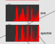
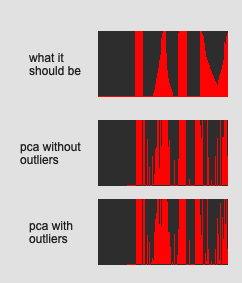
if the patch is handy, try with both at 0 ? I’m super curious ![]()
Not very well as it turns out:
The plain clustering (on the right) is much much worse, and the overall interpolation is mega noisy as a result (on the left).
1 Like
thanks for indulging me ![]()
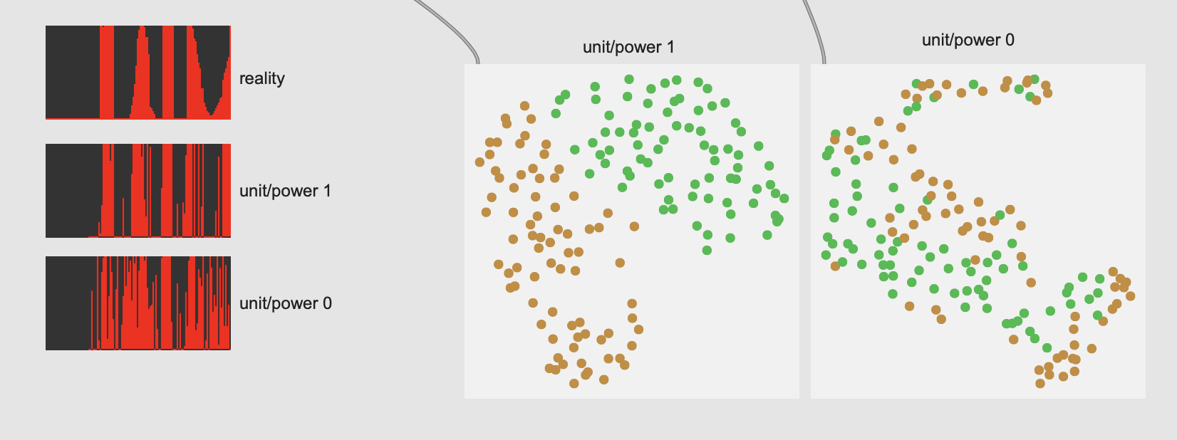
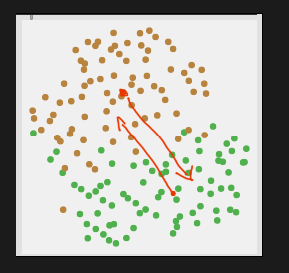
Revisited this idea today based on @weefuzzy’s awesome outlier rejection stuff from this thread.
So as a reminder, the general idea is that (based on a great suggestion/chat with @balintlaczko) each class would be one-hot encoded and then fed into fluid.knnregressor~ where the amount of nearest neighbours would be be used to determine how much of that class it was. If all the neighbors were the first class, that meant it was 100% that class, if it was 50/50, that would be 50% etc…
My thinking/hope was that using outlier rejection to create a more condensed and representative “class” would therefore make the one-hot encoding more accurate, therefore when moving from one class to the other, that that would create a smoother overall change.
I put that hypothesis to the test today.
////////////////////////////////////////////////////////////////////////////////////////////////////////////////////////////////////////
So firstly, given @weefuzzy’s suggestion here:
That I’d compare the 104d space with outlier rejection with the best results I got before (31d PCA of 104d, created by keeping 95% variance).
By going with moderate outlier rejection settings I kept about 80% of the entries.
That gave me results like this:
(umap project is almost identical in both)
Here’s a close up of the interpolation plot:
As a reminder, the top one is a platonic version of what I’m doing on the drum. Some hits at the center, some hits at the edge, then slowly moving from center to edge, then doing the reverse again.
The whole pattern being:
*center / edge / center → edge → center || edge / center / edge → center → edge
Here’s what it looks/sounds like:

(the main thing to look it are the big sliders on the left and right, as well as the one-hot encoding on the right showing how the nearest neighbours (40 in this case) are “interpolating”).
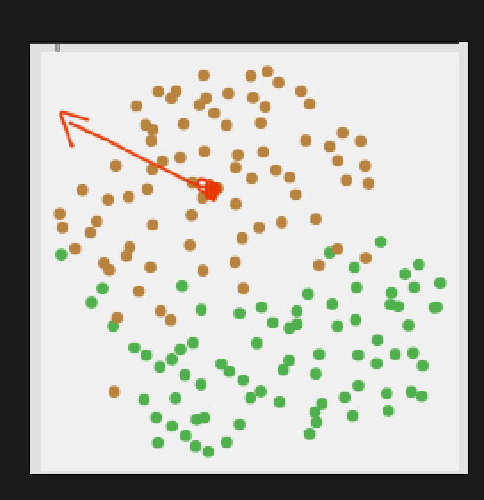
So the initial jumping off point gives me… nearly identical results to what I had before. I figure, ok, that’s a good place to start as this is operating on the full 104d, which wasn’t as good as before.
////////////////////////////////////////////////////////////////////////////////////////////////////////////////////////////////////////
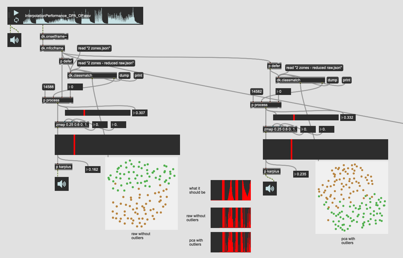
So let me try to improve it by going with the PCA and outlier rejection. Surely that will make a lean and mean classifier!
So this is 31d of PCA’d MFCC (keeping 95% variance) then running that into a more aggressive outlier rejection where I keep ~60% of the entries. And comparing that to the 31d PCA with no outlier rejection.
Here’s the results of that:
You can see that even though there are significantly less entries in the plotter that the separation between the classes is still quite good.
And the closeup of the trajectory:
It’s near identical!
In this one I’ve actually adjusted the scale object range to have a slightly better “dynamic range”. If that wasn’t the case, the plots (and sounding results) are literally identical.
I double-triple checked this thinking I did something wrong somewhere…
Here’s the sound/look of that:

////////////////////////////////////////////////////////////////////////////////////////////////////////////////////////////////////////
Finally, as a sanity check I tried the same but with fewer neighbours in the kdtree to see if that helps make things smoother.
So data/processing wise this is the same as the version just above it. 31d of PCA’d MFCC (keeping 95% variance) then aggressive outlier rejection keeping the inner 60% of entries.
The overall plot looks the same:
The trajectory is a bit varied, but very very similar:
And here’s the sound/look of it:
 vs 13d PCA with no outlier rejection")
So like the others, not very much difference.
////////////////////////////////////////////////////////////////////////////////////////////////////////////////////////////////////////
So my main couple of takeaways are:
- It appears that there is a limit to how smooth this approach can get with one-hot encoded nearest neighbours. Since the classification tends to be fairly binary where it kind of “flops” from one class to the other means that the “interpolation” being shown here is more accidental than what can be extracted.*
- It is absolutely brutal to take apart and process datasets/labelsets. I had kind of overlooked that you can’t use
fluid.datasetquery~on labelsets, which made for a lot more manual packing/unpacking than I was thinking.**
*I still think this is a useful approach, and I’ll include as a refined a version of this as I can get in SP-Tools (unless I figure out something better, more on this below).
It’s not as smooth as I would like, but when working with only classes as a jumping off point, it’s at least “something”, and if being used for something more interesting than walking up/down a melody, can hopefully add a bit of nuance to some mapping.
**In terms of processing datasets. I do feel like some way to split/iterate/pack datasets (and labelsets) would be very helpful. I thought I had already baked some code to do this, but it turns out it wasn’t generic enough, so in order to do all the stuff above, I had like 4 patches open, and was dump-ing little bits here and there manually just to test the results. Really really tedious stuff!
////////////////////////////////////////////////////////////////////////////////////////////////////////////////////////////////////////
NOW onto this:
So after processing how useful outlier rejection would be for general classification purposes, I thought that since the algorithm used (local outlier probabilities) returns back a 0. to 1. for each point, and that it’s possible to
that this may prove useful for interpolation.
One of my earlier tests in this thread was to use class means, and specifically, distance to class means as a way to deal with “interpolation”. That failed, I think, because MFCCs are quite ornery and the mean of a bunch of MFCCs/stats does not represent a useful point of comparison to. And being that MFCCs are intrinsically bipolar, that it just makes for a statistical mush.
Now with this LoOP approach, there’s a more meaningfully computed measure of how far from the central cluster something is.
Now I’m thinking/typing out loud here, as I don’t fully understand if this is possible with the current algorithm. But what I’m thinking is that each class is run through the algorithm to create an outlier probability, and that new incoming points would be tested against both of these probabilities. Then the relationship between the two outlier-ness values (one for each class) would signify whether it is more one class or the other. Something like this:
Superficially that makes a lot of sense to me, but it gets fuzzier when I think about how to determine directionality here, like what if I start dead center in one class, and very distant from the other, but then I start moving “away” from both classes:
So there’s an aspect of that where this gets confusing.
////////////////////////////////////////////////////////////////////////////////////////////////////////////////////////////////////////
SO
This last chunk is more a follow up question for @weefuzzy based on the outlier rejection stuff from the other thread.
Is there a way to implement the outlier rejection such that once computed/fitted, a new incoming data point can be checked against both classes in a way that would offer a smooth(er than I get with one-hot encoding) “interpolation” of where you are relative to both classes?
As a general note, I think this is an optimistic approach given the challenging material (very short analyses of onsets) and one-hot encoded classifier output. Me and Rod have been talking about his data offline for a couple of days whilst I prod it in python as a case study for what sorts of feature and model selection / evaluation stuff it might be useful to add to flucoma in the future. One possible takeaway is that having the option of softmax rather than one-hot encoding might be more useful for this (but also, I think trying to get a regression to give a reliable linear-ish feeling of between class-ness for this stuff still might be ambitious, not least because it’s asking for more sensitivity to difficult data than the original classification).
Indeed
Yes. I have some Max abstractions brewing, which would at least allow us to try out some interface ideas in Max-ish environments. Filtering a dataset by associated labels isn’t too horrible, but also not the sort of code you want to have to write repeatedly. Maybe we can start a new thread and work out what a usefully generic collection of utilities for this would look like.
Seems like a stretch. It can be augmented to score incoming new points (against the fitted data) but the algo isn’t holding enough information about how neighbourhoods of points relate to each other to be able to help much with determining whether a point lies near A, not to far from B but miles from C. That still feels like a straightforwardly supervised regression problem.
1 Like
Interesting. Is that something that is doable with the kind of outputs the NNs in FluCoMa?
I’m not married to the one-hot thing at all, just after this idea of trying to create gradients/interpolation, with the one-hot thing being (by a large margin) the best results I’ve gotten trying to do that so far.
By supervised regression problem, do you mean just training the individual points along the continuum? Or does that mean something else in this context?
I did do some testing with multiple “in between” classes upthread with not-meaningfully better results:

I think back then I landed on 3 zones giving the best results given a reasonable faff-to-improvement ratio, but my hesitation here is that this would create a separate training/plumbing process than training individual classes (or loading classes that have already been trained).
I don’t know what the Sensory Percussion software itself is doing, but I want to say I heard a podcast ages ago where they mention using the latent space for interpolation.
Looking at this paper from AIL on classifying percussive guitar hits, they talk about latent spaces as well, but in the context of VAEs, which as far as I know, we don’t have access to in Max.
Here’s a (very short) video example of their results:

Sadly, much of the paper goes way way over my head in terms of technical detail/theory, but also the use of CNN/VAEs mean that I can’t directly map what they are doing in FluCoMa either (though would be nice!).
Not yet, but I’m mulling the advantages of adding it as an option (this is partly informed by me combing over your drum data).
Essentially yes: we don’t know how ‘linear’ the input space is, but the idea is to get an output space that feels linear, yes?
Indeed not, although there’s nothing that magic going on there: the idea is that the hidden layers of the network have learnt some useful representation (so, automatic feature learning) and one can use that learnt representation as input for a further task, like classification. Not clear that one really needs the ‘variational’ aspect of VAEs to do this.
I’ll probably have more to say about this as me and your drum data get better acquainted…
Ah cool. Probably useful in a couple other contexts as well I would think.
Gotcha. Yeah that’s sort of the multi-class interpolation idea. I guess it localized each clump as it went, but the tradeoff was that each class was less distinct/accurate given how similar they were.
Here are the relevant images from upthread:
By the time you get to 5 classes it gets to be a bit of a mess and although the space is more divided with these classes, each one overlaps so much that it doesn’t result in much of an improvement.
I suppose if the overall classification is improved that would change the calculus there, so I’ll check that approach (labelling the “in between” classes) if/when the core classification is improved from the tests you’re doing.
I guess that automatic feature learning requires much more data and/or complex networks to happen? It does sound like it would be a useful thing to be able to do, even if it doesn’t solve this specific problem.
Plus, it’s hard not to be dazzled by the shiny stuff one can’t immediately do.