Sorry this is not necessarily a code share as the code is a bit noodly right now, but here’s a project I did last month using UMAP and a Traveling Salesperson Problem solver to organize audio slices into 1D paths and the reconstruct them through time.
I started with a bunch of audio and video recordings of some music that I composed.
I sliced all that audio into 100 ms slices.
I analyzed those slices and extracted audio descriptors (714 columns by the time the 1st derivative and all statistics were done!).
I reduced that to 11 principle components (and was able to retain 99% of the variance!).
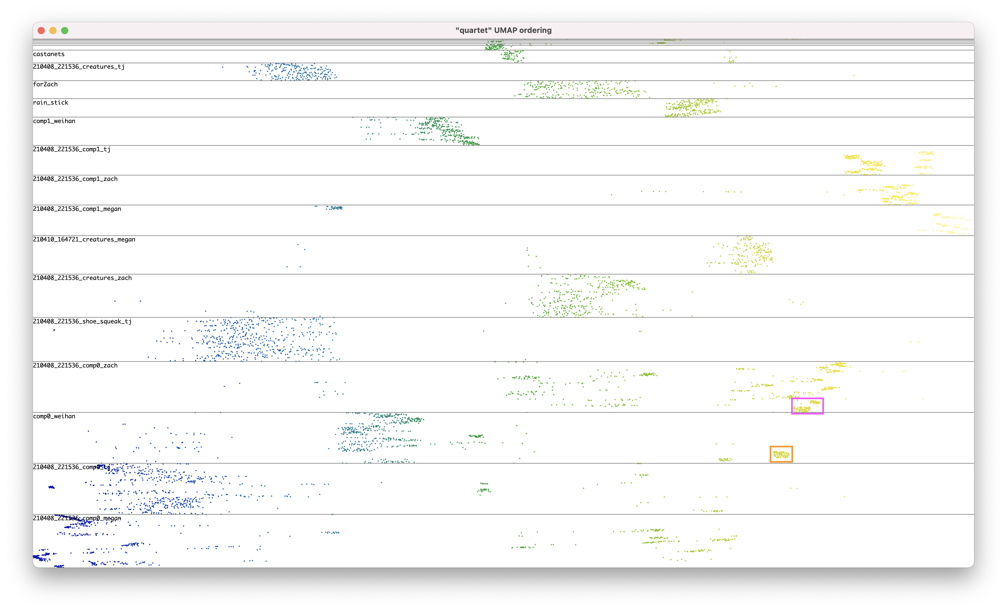
I then used two ways of reducing this further to 1D, the first was a UMAP down to 1D and the second was a TSP solver algorithm (in python… python-tsp · PyPI FWIW)
Then with each of these 1D sequences of slices, I reconstructed the audio-video file.
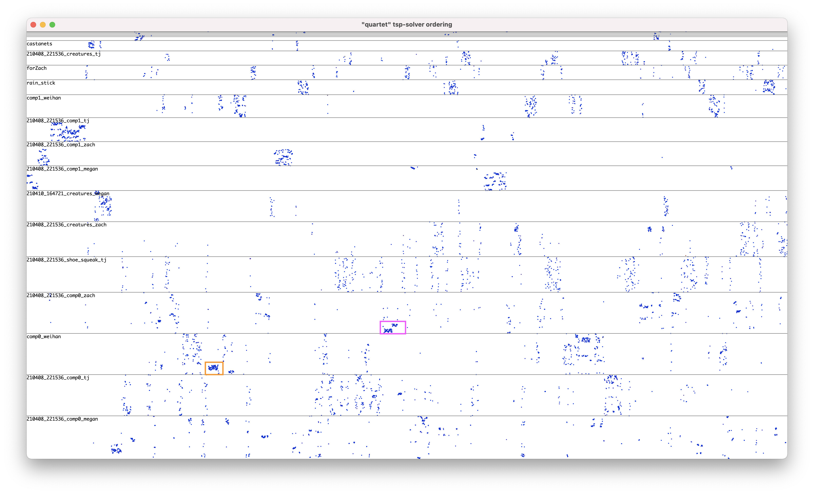
The tsp-solver solution is quite jittery, frequently jumping between different audio files and not staying in one place for too long:
One can kind of see that in this plot. Each dot is a 100 ms slice of audio. The X position shows the slice’s time position in the reconstructed sequence (the youtube link). The Y positions shows what source file it came from and where in that file (bottom of the “file’s bar” is at the beginning of the file, top is at the end).
While creating the final piece, I selected some passages from each of these but didn’t end up using all the material, just the passages I liked! You can watch the whole thing here (password: framerate). The piece isn’t supposed to be public yet… so it’s behind a password…
I hope it’s interesting, maybe creates some ideas or inspiration!
This is epic, thanks! I’m on a train so I cannot watch the videos yet but I might tease you in the other thread r.e. your last paragraph here What I like very much is the transparency of the process, where data mining is investigative and put against itself.
A few thoughts right away, on the more ‘objective’ matters:
#4 means that you had a lot of redundancy in #3. But @groma will confirm that what I say is true.
I’m impresse by how well UMAP has fared - I presume you tweaked the local-vs-global topology priorities a bit? Could you share how you manage to tweak it?
were you not tempted to do a more perceptual segmentation? did you try and abandoned? I’m very curious about the investigative process, where you stalled and how you curated that clean list. Maybe it was just as is from the outset, but maybe not?
Yes! So PCA was an important step! Lately I’ve been doing a lot of big analyses like this and then letting PCA get rid of the junk for me, especially since, in these cases, it doesn’t so much matter which raw descriptors are most influential, really what I’m after is the variance between slices!
I did no tweaking, I just used the Fluid default values. The output was really compelling so I ran with it!
I didn’t try perceptual segmentation this case. I did that elsewhere in the piece, but here I wanted to have it be more temporally consistent–like the section was clearly a tour of the slices, of the sounds in the recordings, without the capital M-Musical content they would convey. That way the musicality of the section comes out of the sequence of slices, out of the algorithm, more than out of the musicality of the slices’ content.
Also, I had done something similar before, with just audio, not also video, and liked the results with 100 ms slices, so I was following after that.
It was pretty much as is. Like I said, I did something similar previously (a few years ago, actually I think you and @a.harker heard it in Chicago?) so I was essentially recreating that process with the Fluid tools. That first time perhaps the list was less clean but I don’t recall the investigative process from then to try to retell it.
This is super cool in general. I specifically like the travelling salesman restriction.
This is super interesting as well, and though we ended up chatting about this in the last Thursday chat, I wanted to bump the thread version of it.
I’ve been chasing that dragon of having conceptually meaningful sub-groups of descriptors (LTEp/LTP) but that gets problematic when you’re combining sources in which some characteristics aren’t as relrevant/meaningful. For my case, this is often pitch, but if variance is what one is after maximizing, it’s possible that it may not make sense, or be sub-optimal to conceptually group things ahead of time.
Maybe some kind of hybrid approach where you have a reduced descriptor/statistics space (similar to what you have here), where it doesn’t matter what’s in it, it’s “a good representation of the stuff”. And then along side having some perceptually meaningful descriptors (loudness, pitch, centroid, etc…) that can be used to bias/skew the query (e.g. return the nearest match from the pile of goop that also has loudness > -6).
That’s some (more) functionality that isn’t presently possible with the querying tools we have, but having a kdtree that can also resolve parallel logical queries (e.g. find the nearest neighbor from columns 5-20 (which have been pre-fit) && some other query on column 2).
Oh yeah, I remembered I wanted to bump this bit as well. From our discussion you mentioned you had to pull some numbers out of the .json and manually compute the variance.
I could be wrong here, but it sounds vaguely familiar that this is something that was going to be added (the ability to request an amount of variance, rather than a specific amount of dimensions). Or maybe that was the error value being returned from UMAP or something else.
Either way, this seems like a super useful way to use PCA such that it would be nice to have as a native feature, or a pre-baked abstraction layer to get to the same results. Perhaps this is what @weefuzzy was building towards with his variance/novelty diagram stuff from a bit ago.
Yes, I gestured at it, although the main focus was on plotting the correlations between input features.
Getting the number of PCs corresponding to a proportion of the input variance is easy enough using the values from dump, because these are always properly ordered. One just needs to accumulate the list so that it goes 0-1, and then find the index that accounts for the requested fraction. Here’s something quickly hacked from my own personal abstractions for doing the list accumulation and index finding.