Intelligent Feature Selection (with SVM or PCA)

[tedmoore]

@rodrigo.constanzo

Or do you mean something different?

I’ll try to outline what I did and how to do it from the FluidPCA. That way others (looking at you @rodrigo.constanzo) can try it and see if it seems useful.

1. Do a Fluid PCA fit on your dataset in question with the numDimensions = 0 (scale first!). This will analyze for a number of principle components equal to the number of dimensions in your original dataset.
2. Get the values array from the Fluid PCA dump. Square all those values and sum them up, then divide each of those squares by the sum. This array of values will be the weights to use later.
3. Using the bases matrix from the Fluid PCA dump, first (a.) transpose it (asterisk for @weefuzzy below). Then (b.) convert all the values in the matrix to their absolute values. (c.) For each row, multiply every value in that row by the weight from the weights array that has the same index as the row (all values in row n are multiplied by the value at index n from weights array). (d.) Sum the rows, so for example matrix

[ [ a, b, c ],
  [ d, e, f ],
  [ g, h, i ] ]

would become: [ (a+d+g), (b+e+h), (c+f+i) ]

4. If you want to keep k raw features, find the k max values in this resulting array. Those k indices are the indices from your original dataset to keep.

I hope that makes sense. Like I said, my tests say it performs better than random, but I haven’t tested it on much. Also it doesn’t perform better than using the k PCs you get in the process anyway, so it’s only worth investigating if it’s necessary to keep raw features.

*@weefuzzy, I’m not sure why this is the case, but my tests showed that this was a necessary step, also the signs are inverted when compared to sklearn? I don’t know enough about PCA to know what these differences mean.

//==================================================
Pictures from testing my port from sklearn to FluidPCA:

//==================================================

[rodrigo.constanzo]

Awesome, thanks for the detailed breakdown!

Other than the *transposition thing, I think I’ve implemented this correctly, however, my results are a bit weird. As in, I seem to get a nice orderly pattern like this:

ImportantFeatures: MFCC1
ImportantFeatures: MFCC2
ImportantFeatures: MFCC4
ImportantFeatures: MFCC3
ImportantFeatures: MFCC5
ImportantFeatures: MFCC7
ImportantFeatures: MFCC6
ImportantFeatures: MFCC8
ImportantFeatures: MFCC9
ImportantFeatures: MFCC10

This seems pretty unlikely.

As a point of reference, here is my previous version (which I’m sure has stuff wrong with it):

ImportantFeatures: MFCC8
ImportantFeatures: MFCC10
ImportantFeatures: MFCC9
ImportantFeatures: MFCC7
ImportantFeatures: MFCC13
ImportantFeatures: MFCC11
ImportantFeatures: MFCC16
ImportantFeatures: MFCC15
ImportantFeatures: MFCC12
ImportantFeatures: MFCC17

Looking at my dataset, the values are massively skewed towards the results I’m getting in the end (with the weighted sum). Here are the values for my test dataset (attached below):

  "values": [
    673.8362958342209,
    338.6515716175081,
    260.5718722831362,
    228.3479775847835,
    161.27948443092583,
    137.3968786415179,
    130.18460519211504,
    117.8497815323449,
    106.45463928836723,
    97.96113750682099,
    87.04047077667117,
    85.19806093624975,
    77.16552071744412,
    72.7289747754491,
    66.65032492000918,
    62.996468347624074,
    58.49098132121391,
    50.31602507677747,
    44.452909961833726,
    31.008415770540466,
    18.333930137956433
  ]

Which after squaring/weighting I end up with this:

0.547614 0.138316 0.081888 0.062887 0.031371 0.022768 0.02044 0.01675 0.013668 0.011574 0.009137 0.008754 0.007181 0.006379 0.005358 0.004786 0.004126 0.003053 0.002383 0.00116 0.000405

So in looking at these values, I can’t see how I’d get anything else than what I’m getting it now, if I apply the values as weights further down the line.

Either I’m doing something really wrong (quite likely) or these values aren’t behaving like I expect/anticipate them to, or the transposition thing is unbelievably significant.

code_dataset.zip (350.1 KB)

[tedmoore]

@rodrigo.constanzo

or the transposition thing is unbelievably significant.

It is! Basically it makes row 0 become column 0 (and vice versa), row 1 become column 1, etc.

I like to think of it like if the matrix were a sheet of paper and you keep the top left and bottom right corners in place but flip it over.

Transpose

[weefuzzy]

@tedmoore

*@weefuzzy, I’m not sure why this is the case, but my tests showed that this was a necessary step, also the signs are inverted when compared to sklearn? I don’t know enough about PCA to know what these differences mean.

Yes, we store the matrix transposed relative to sklearn. Nothing to worry about (once you know it). Sign inversions are also nothing to worry about: different algorithms for doing the Singular Value Decomposition that both we and sklearn use to get our PCA throw out the signs in the bases matrix differently, that’s all.

[tedmoore]

Cool. Makes sense. Thanks for the quick reply!

[rodrigo.constanzo]

@tedmoore

It is! Basically it makes row 0 become column 0 (and vice versa), row 1 become column 1, etc.

Riiiiight!

That makes loads more sense…

I was picturing that meaning offsetting the values by x amount… lol.

I’ll have to come at this fresh tomorrow as that seems like a fiddly operation in Max land and I’m giving a (late night) talk for UChicagians @spluta & @tedmoore in a few minutes.

[tremblap]

@rodrigo.constanzo

I’m giving a (late night) talk for UChicagians

ohhhh is that online anywhere for other parts of your fandom to enjoy?

[rodrigo.constanzo]

It didn’t look like it was recorded, but that’s a question for @spluta.

[spluta]

It was a great talk. Thanks so much for doing it Rod!

[tremblap]

@spluta

It was a great talk.

tease!

[tremblap]

Now on the content, there are a few unknown for me in that discussion, mostly for @tedmoore

• when we spoke about all this, I was pointing at normalisation of data ranges as being probably a quite significant aspect of it all. The range of PCA linear transform will be quite affected by the range of the data if not normalised, yet normalised MFCCs (scale and curve) between themselves and compare to pitch and loudness will be quite instrumental in these transform… so I wonder first how you assess the multidimensional clustering and make sure it is valid as a way to assess you data and its range/transform/sanitisation?

• another interesting comparison would be for me to see what you get if you ask right away for a redux of the desired size by opposition to curating, especially in labelled settings like these. For instance, an MLP would be good and quick at sorting what is needed and what is not… training is long but query is quite quick… Even unsupervised, as autoencoder of all the dimensions, it will be quite efficient at dismissing the noise and making a relevant bottleneck.

So I’m curious - because I’m stuck with similar problem but I am tempted to use non-linear MLPs to curate dimensions in both these ways instead of selecting features à la human…

[tedmoore]

@tremblap

another interesting comparison would be for me to see what you get if you ask right away for a redux of the desired size by opposition to curating

Yes, using a PCA to reduce the number of dimensions to a desired size does perform better than this “feature curation”. So the only reason to pursue this curating would be if it is important to keep “human readable” features (which I think is the initial inquiry/goal from @rodrigo.constanzo).

@tremblap

so I wonder first how you assess the multidimensional clustering and make sure it is valid as a way to assess you data and its range/transform/sanitisation?

I’m not sure I understand what you’re asking? I normalized the data before the KMeans and the PCA (and SVM). I wanted it to just be “data” in the abstract to do some testing. My test was just “If I do this feature curation strategy, will the resulting subset of raw features perform better than a random subset of raw features?” The task I chose to test performance was classifying labels (created with KMeans).

Perhaps it would be good to test it with a dataset that has labels that are not derived from KMeans as a way of checking if the KMeans labels are influencing the result?

Also, if pursuing this feature curation strategy, I think running various tests like this on one’s data would be appropriate to really know the data–and also to test it on the task it will actually be used for.

[tremblap]

@tedmoore

I normalized the data before the KMeans and the PCA (and SVM).

This is where my work lies now. I am fascinated by the (huge) impact data pre-processing is having on the quality of anything that follows. Log vs Lin and relative range vs relative noise.

@tedmoore

Perhaps it would be good to test it with a dataset that has labels that are not derived from KMeans as a way of checking if the KMeans labels are influencing the result?

Indeed we have labelled data to do such test - for instance in the papers we have some of the cool @danieleghisi curated stuff from orchidea (Computer Assisted Orchestration - #11 by tremblap) you have in the name some interesting human features that @groma is using to validate. For instance, the violin pitch, its timbre-via-technique, and its loudness. This is quite fun

[tedmoore]

@tremblap

This is where my work lies now. I am fascinated by the (huge) impact data pre-processing is having on the quality of anything that follows. Log vs Lin and relative range vs relative noise.

Yeah, I would be very curious to hear what sort of heuristics or intuitions you find after picking at all these differences.

@tremblap

labelled data to do such test

Cool, I just downloaded some of the Orchidea datasets. I’ll see when I have some time to run some tests and report back. Thanks for the pointer!

[tremblap]

@tedmoore

Thanks for the pointer!

have a skim at @groma 's Fluid Corpus Map paper so you can see what he did there already…

[tedmoore]

@weefuzzy

Yes, we store the matrix transposed relative to sklearn. Nothing to worry about (once you know it). Sign inversions are also nothing to worry about: different algorithms for doing the Singular Value Decomposition that both we and sklearn use to get our PCA throw out the signs in the bases matrix differently, that’s all.

I just had another thought about this. I don’t know how much it would change under the hood, but it may be nice to have the key names in ‘dump’ be more descriptive as to what they are, or have that information in the help file or something somewhere. That way someone coming to the tools who might be “looking for” the eigenvalues for instance can quickly identify how to get a hold of them.

[rodrigo.constanzo]

@tremblap

This is where my work lies now. I am fascinated by the (huge) impact data pre-processing is having on the quality of anything that follows. Log vs Lin and relative range vs relative noise.

Curious how to deal with this when it comes to secondary/tertiary stats (skewness of the 2nd derivative of loudness, etc…). With things like perceptual descriptors, or to a certain extent MFCCs, the scale and boundaries are semi-sensible, just different from each other whereas some other stuff gets fairly irrational right out of the gate.

I primarily ask as one of the main things I’d be interested in “representing” is a sense of morphology, so derivatives and related stats I imagine being of significance in capturing that.

@tremblap

Indeed we have labelled data to do such test - for instance in the papers we have some of the cool @danieleghisi curated stuff from orchidea

I’m curious what makes for a good set of labels. Last year I made some training/testing hits with my prepared snare stuff so that I can test/compare, which is what I used for all the stats/verification I did in this thread. I tailored it to my intended use case where I have single/individual “training” hits, and then 5 separately recorded “testing” hits, since my approach (at the time) was more about building a kdtree with loads of individual hits which would act as “classes” which the knearest would give me the nearest match for. I did it because I wanted an arbitrary amount of “classes”, and only wanted a single example of each.

For the purposes of testing I created 34 of these (as in, 34 individual hits, and then 5 addition hits of each 34, so 170 “testing” hits).

But I guess in general it’s good to have samples where the names of the files have symbolic meaning? (instrument, pitch, dynamics typically).

If so, that makes me think I should be able to harvest some great test corpora from some of the sample libraries I have where I can break off sections of it based on instrument (“spoons” vs “crowbar” etc…).

@tremblap

an MLP would be good and quick at sorting what is needed and what is not… training is long but query is quite quick

I have it on my list of things to test again, just to revisit the speed “problem”, but curious on your thoughts/experience with regards to pre-fit PCA vs MLP as part of a process chain with regards to how fast they are. I guess in both cases they get broken down to multiplications/calculations, so it’s just a matter of passing the data around.

As @tedmoore mentioned, having some legibility, or still perceptually-meaningful descriptors in the mix is definitely desirable as you can then do perceptual querying ((loudness > -10 && centroid >= 20) && knearest) which would be impossible if you boil everything down to abstract/reduced descriptors. But at the same time, I’m not completely averse to doing some overall descriptor mashing (if it isn’t (much) slower than not doing it).

[rodrigo.constanzo]

@rodrigo.constanzo

@tedmoore

It is! Basically it makes row 0 become column 0 (and vice versa), row 1 become column 1, etc.

I’ll have to come at this fresh tomorrow as that seems like a fiddly operation in Max land and I’m giving a (late night) talk for UChicagians @spluta & @tedmoore in a few minutes.

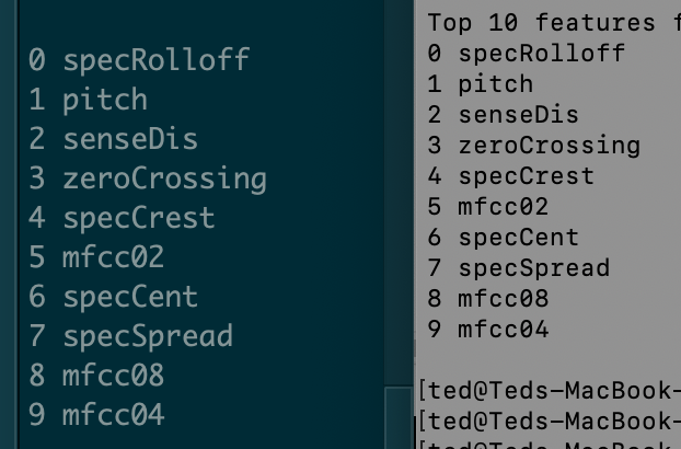
Ok, tested this today and the results I’m getting are the same:

ImportantFeatures: MFCC1
ImportantFeatures: MFCC2
ImportantFeatures: MFCC3
ImportantFeatures: MFCC4
ImportantFeatures: MFCC6
ImportantFeatures: MFCC5
ImportantFeatures: MFCC7
ImportantFeatures: MFCC8
ImportantFeatures: MFCC9
ImportantFeatures: MFCC10

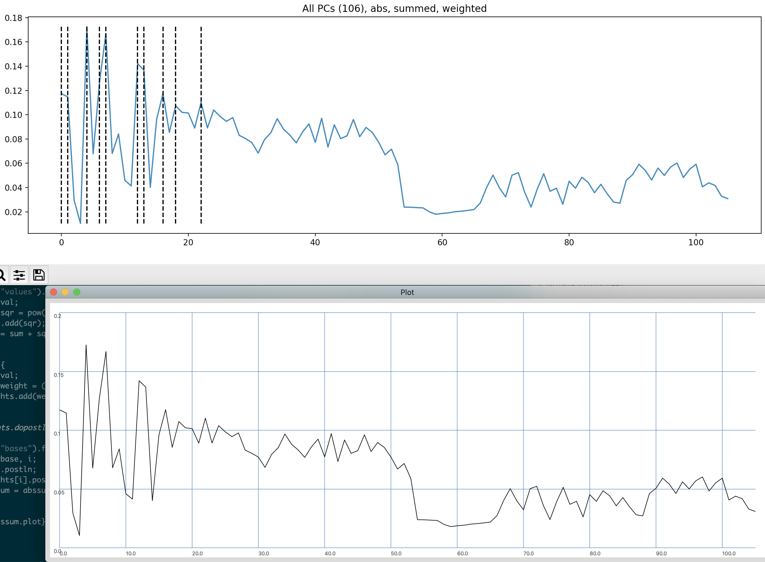
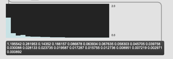
I seems that the values, as they exist in the dump output skew so heavily towards the first entry that transposing the bases matrix (via jit.transpose) had no impact on the overall results.

  "values": [
    673.8362958342209,
    338.6515716175081,
    260.5718722831362,
    228.3479775847835,
    161.27948443092583,
    137.3968786415179,
    130.18460519211504,
    117.8497815323449,
    106.45463928836723,
    97.96113750682099,
    87.04047077667117,
    85.19806093624975,
    77.16552071744412,
    72.7289747754491,
    66.65032492000918,
    62.996468347624074,
    58.49098132121391,
    50.31602507677747,
    44.452909961833726,
    31.008415770540466,
    18.333930137956433
  ]

As a sanity check, could you (@tedmoore) run your process on this dataset to see if you get the same results, as I’m certain I’m messing up something somewhere, specifically at the values step.

test_library_20pl.json.zip (344.7 KB)

These are the columns in the dataset

0, MFCC1;
1, MFCC2;
2, MFCC3;
3, MFCC4;
4, MFCC5;
5, MFCC6;
6, MFCC7;
7, MFCC8;
8, MFCC9;
9, MFCC10;
10, MFCC11;
11, MFCC12;
12, MFCC13;
13, MFCC14;
14, MFCC15;
15, MFCC16;
16, MFCC17;
17, MFCC18;
18, MFCC19;
19, Pitch;
20, Loudness;

Here’s the updated code from before with jit.transpose added in.

----------begin_max5_patcher----------
4561.3oc2cs9aaijj+yN+UPHre3tacz0uereZdr2L6hKYufalCCNDrvfVhxg
ITjBjTNwYwl+1u9AE0KxlMkaKo4R.raKSxtqp9UO5ppl9e7palbewWRplD8m
hdezM27Od0M2X9H8GbSyOeyjkweYVVbk4xljm74h6+3jas+p5juTa93OlVOs
tLNuZUQUxlea95ko4YI0l6D17gqhqm8gz7GtqLYVsclQLwTvsQDBV+Mt4qHz
TPzeu4dRmalD0D+ZzNO7h00ad5nlO09Q0OsJw9n0Kr6VFWWl9kI2FMYRzeWe
c+yW8J8Wt84QyOl7kUkQ+gEvn+M0WQcR0n9oZBvP0LHbJhvPbNv7OnDpndfS
l.DP6lM.6iMDTBuNJKJ6DExXLW+MJcJ0E8QFoXN3B2ulEUsd4nkoTtltHR4T
HiHgDtTPvLNDo9vADofKMIuOdFNVAbCdlPkGimELWztTdIQyaI6+csZbz2UM
KNKtbYw7jH3IpTSwcvDfbjKtffcI4BySmUOcc9p3YeJ5w3r0IU+oSE.fvSIR
DkRrzNVn.+PkUNGzNWdoo8STPiE7iEzTfKia7drcS5iV0Kuzh73xmLp721p5
2bCUwOlL+N0iVs3tKtV4q6900Vu52zxHtYRxx6SLqBvsMexp3x3kI0Ik2kjG
eeVRO+xkwqV09qM+VCaerL+kIUUwOjbD2+yko0Iik8ioLCOFBlBDPLSoaQ4B
HiyTxDhy.HPmEn1rhkKSxqOhZiUyYdcTwhnUIwepJptHpN9SszeVZdxL8UrK
86qBnhO.zjNDY.fBf0ga27AJra9.HfhV5XEqPLhZo.qCCoKEIB4rHI6i3ffQ
ScHgvepCeQwoKRhqWWlTEklGU+gzpn4w0wUI0ABnBrb.hILPNyEPEiBGPsOp
UIC17YKJxqqR+pgqJmBFKkob.Xh.rIZOiWOHuGSQhWdJCDZJiRPdPY3WdJid
+znYYIwkQwKTtohRhm8gn0UgwTpjXiWAZrgJbBPQvWdhst7onEokU0pu9Xxs
QEJpNKS6Fo9CIKCCICHaoUA1EECOC.W5T8FvhVUllOKcUbVj5BWUjqtzJmj6
tnbnXzvbtzHwsheHEZinsG1.aWUqbU3Rle0eII6wj5zYw8vj14dVDOytPCHi
i7RpWPswcwn3o7i1jG2Ilg9xiYHSilud4pnp50KVLIL.BjhfnZKcRqqaqcAR
ODI9ZDQfmprZjOORMkQySUWRkd6DYo0O8RpIAAFGEXIoisCRDNUrPWirQzzn
28ieeTZcfPVPnQgARr1cQNAVvqQNBbZTYR7baLhIQOnbMkGM8iUE4gkE0riN
nzEKRdI4P8sIAznyfjvlkH6NEbuEA1Ec+OidycBL0WJ6hld6uloP0OL9M2Yy
YOgZyKjyzcItz45UGVUczeUEQUYcbd8O0rauwlxOHxtecLQZyCCBAfTFlvkJ
CaXmY7lyCW.A8KIS0g.AGuvzRWHfw9Cg6jPXWZoYoZJRhpdZ48EYmJoh0g+e
Xpz3NIbl7RS3yJTaBZwyD7hrQ46ttiL7HyZa24pUufuSmJkCyN61nufax.6l
K68lKr8RU+lOk7zt4pU8IlT12Lyu8m9weD1vluYCStyG.r+G.xqG.p+G.1qG
.t+G.wqG.o+G.0qG.s+G.yqG.q+G.2qG.u+GfvqGfn+GfzqGfzAPB3GRxEVz
SvnCzHzO3HzAdD5GfD5.QB8CRBcfIg9AJgNPkP+fkPG3Rne.SnCjIzOnIzA1
D5G3D1C57coJK59YkpGv4aJVOOOQ6gY6CoYn5ocZEWq058JkilT8FsM1HN8x
l4JH0GOUm8MUf.6z8NUbMzDFYoyRhNkZszPoL5wQlJbVHdJ+ZftUAlepaAQP
2lBydIRvUQraGmT2Q1sABkX9nBvKotHchHHgxc5kcOPVF5svjSAR.A.i.SQR
L.QUCTgyiwPy.DPp+D.kifB8.lDSLCnX0l.LCT2NVOfPoHjd.lRklAHoRIxL
fRnLy.BRx0CfB.xNPplNy.NtY.FJM2kZtElo.nDXlaGfEMCzUXpyDRhOsDMP
Yl7E0TvJ8NT6DMvOK4ZPgMp2lVrQVMhlTlPbk9KxXyYx8w4OrEM2YufDNk80
eMMZzILpg5gHibj4rsNH8TkXrSx+1seOUi0BZSRd+3aRxM8DZW8Pms7q8R+v
QZOeCcG1jBNZ+zTnIQfbkmqi6BV2MHA3Rljv+3I2afbBYrjJdr1nBMX9iEo4
mJ4JviEKiuno+031IorSxkNL41EPl4LTLLYjwinkt6DRxIKr6SI1T83STQtS
SWXmwigwWVw8yJLzlXMZ5sW2AdhA++6.OOIbSSamffcrOM23Fz4oogWtNqNU
sMz48XSXyzUkTq9T0sZmMSnK6tx6G7zzrXXp4aPHqG5cf8kpV.U0OYCcqcQ0
T6UDbf80E3v.Osvc2fEnjgi2EwtJh28DiqWXZ7Qrj6AgRtlCrOqHdt1dPDv2
+ehfBL.zQXSbfSKDfKZExMEYczIwgY7jvrInyYhptr8+rtyOFMwY6mCVa+T5
vY4kLnfEYqSmOsokm+Vzqe8qMGtwzjdjmdzkO1NdFRbJQgm3lXWnTCqegNPX
w2W8u7GV.+WG8A9qI6Kvia+KA08QgS96tS2Xim7FC5Bt6S2H954n98GOkit5
Fp0V3bgvszDdIkl1ViPEje0nsUIM1mnJ+NGAfcugNw4quH5MT7Sffs9RIfN5
WSrS2rBwEtcsdPIkWE8ceMSc85HdU9MAfQmJpFCVB3TNVHvPK8S4XkYagSeU
hKtBc.cX0.CnftZaWmdu3nqJ2W52IAUqRUau+6xRqTSc9C0evAzXXeYJSAJ3
fTWCE8dTEL8o5cf5rgtNZNLcewOZEBVSqZxr4szIcRt317NERDC1dNeNr42b
KXYWzzO+wpnUyhuSSxSUiuWo1WcpuQF55HLCQNk1rSvm93xd0hTk95ll3dGR
chyCub3yo0hz5gslN7NdZxOn8Pjz6VdjW987nX0eK56Tye6AEopmB2M7ddPT
PGcEr6sriYizGh1zd.7gnQhqSmL9SbculOfTmBaRqvVO0VAytbc2PAsT6tOm
Nu9C1Vmi1dzJF.jXVJlxqevq8GC0o+78YRUEqKms4Q07B3IZKAMOopNMOttI
oxueqSO8E0obv2IRaiYvYJDSj90OxfSj9sywNWTQoNcv8dXQB5Tad0vz0bCd
VysvKxVEYaD7Yxf06OXvYhGBQ4ARo93mzPPTXumpmKUw8QRsAJ87lIejTTPH
lIejTLbHlIpOnufv8zPXzPZTgXlX9fHzGvlm+L4CLmEDZB3wLgYgXl7Xhz8S
zy1FA0K0oPHl17PbCHBAySuQOOr6QBwTg7ZpBA3yXSCNjjRDhY5bA9Hxyk9D
waZ5YOSDeUnd1bO7YalPd.83g.5Q7w+DNDd20ci3fzDNDggQ7YWB3PXMh.7c
lPO2YxGydAfhvmMKDXebOgCQrxlk6PXbZHvCXur5EB8VrO.BbHBi.iGAME1s
B62T+hrSXLvq3LBhJ2YR0F4ipMJDp1HehlFEBmJHz4xbExe.wy0+Ua3qCmFF
vydp7xhELHSEwmfZnAapFbGpggp7Q80DpFLzlG8atI78l6koyWUjlW2jpWAg
Xd2DhMsmBDy3s+XnMo52xEw61bNJ.yMzW02t4URn8s4hsxuRJeJhdzOhIlZY
nu1M+zyFh4UVuIuDdf8atOTxFL.Cv2rvC6nfFwqV8XR4lda2LKSVF+whx12O
BJAbt8GM0PYRYxis8Bu8sWvj3xYeHsNYl9sIhofLegYqp8D8KC7x70oMLYyo
CehoYqOnJJskr76WOOs3WpiqWWc2aSxWaKmihrVDuNqdelw8OrHMKaVQlc8s
aYP2TGmI1e6ssusPZt12aNjmDHTnXdSwPLGwLiTCnzcv2M2CbyMQnDI.ouTc
oeITyHABSw5QfCtMz14B.k1Y.HE.hcj5iz0Ld2aKN+AaMYssna6IPnP+FGpg
sqtUY60utt3gx34lZrdTobusAKUpOhFa5w8IM7TSC5u4d1E60JLdy5Mu+u5V
.rG6jvoPrgefjXgzNhBAL4djnWRsVJpGAmmLy8EchVAlfCnBgcjff671ZEcL
pZRzWKS+Otcj8I8hH4ZOUBYIl2e46Q5bjheZVMPFGYwbB..RNjGu2cIADntF
xJ5URIbCMHzG+XC2fxZuu3YyTql8tWLRg3MbXxFFgVGgbfTc2WdbJiN+WqRx
i9k37pneIYY58EYy21ICJBa4gyBWnXsVYC.JD1QpIDg1eZz0u0bi2klqMbkz
hIvRDjYwbazPQ6JbChBwaiqqcoPr6qsO8axwCXPadS489s1helKn28802YtM
f25oRp1vmUvS3.COSqFgOPhZNUR6bmlt5Qc6J7C0pOnTiLM42uiUt891Br18
A.EjKcWKs20nc47cn55mkqCUc+9xz3rICqwYPCa9R3Tw9se8m7FJC09ss1vz
3WiROeiG7qAToeFOu3AKzMnTzOnDxvJaGF2PbBSJaFAjChIo.NyPP.FECsOB
HBhb6N4u7z7xhGRx+UizxkiDBCp1utIpLIhQLbQpDpzo2eBZiudewrNRPiWU
0ZhxrhNscACzRFHHto6oRm4ejUMVm6ZzXg4cDO7VanXI2ZADKabQn+HJNLn0
8nIQq+5iGcRXbWPYY+HY+n4tPx9JUN.J+yI4IOFOY.f3wFWuPliavp+vNGWy
AQrMQJHZAFflQAeY8m0tpt1VT+bbZ927V4F25453QgeoU8Yya+MGKtiP5vF.
01u7hrlPWUKp+ycO359gsNX03bab9aQ2OqBc5Ibn4Hj7q2jLeb5g9RErWTyZ
u07W3xY0kYOiUePWP5Ny+atS503LebsfP9aEy2bTK7vpnmgG3vO+kmfGkIjW
ZG3+s0Ku28hoKKUG6z7EXo8tzY0Cyqt3xy2Ulz92wqqnnM9kYEqR7ObisYsV
h0+qCyvGXg4rxj+036C91h5B4Ln8kfRTpX1uezAP2c7DcrQjWVCG+ZwC5MfE
rvYcHTvbFgCs2AACM6jjzTVkPRR+OKGnvRmw.M+s3GSVTTt7aAmCO9HOA55Y
GDhadb4mdcd5Cen90l829bqhW2ImCN.vI3IsH3Ila+jVzt29Qlc5tLJ3aV96
N8CjVih71hozVVEg4wDHjxGMKfjRvlW2Eg3Q4bujGVWCmYoEDvzq42z76Bj5
ggcS6sXB2mkn76YKE3OTT7ogR701ZVbz.Pvfbo4exaysLESCHZcwhY.kBn6J
ksagILWNd2QAHis9u1NiVJOK0+1CowQVQ83dNLovmtcWOlrNSywv2Ve5K2t2
WCW.Jextmre6Cs+YF+xErTlNThgCg9vbi.jjl9PQJwBdyHtviMHvZc2QasQu
Q4Ibz0x3uvzmudeooCXvfcL71AVTr+9a3M5uWxxInIXyaH.+2kGBSQx8cVp0
NCtbXu2jEuXgpJZKE+wibXElKz8X1scN5LFEfm1tCDpZesC+jh1WiCiKoa6z
SeAOuF1WZH+P15jMujB8rBG5tRj2Tj8sFijA2DTyBrr3y4idEddLRZWg+3Sw
ieAp+ytgsG.3bLFY01PPU3YgeA9ykIImvJzv8ZSEGjoi8H7Kt2prrkWGO5km
f.XLaRBY.0hyvJYRnjF903+cx7Qu93sQwBa2TEnwiQnWe+uIYYEe18R7395h
JA.gSuzHpsOX3BnvDZt5dnD5KFAf98HAXJewOWjcBPj17ePUQBQssbztNACx
Bb05xUYIiJ3TBvFWChBXRCFFInLjvyHz3ssCHARUlML11zVOBJiuLYVR5itq
bWWXh18MscwA1s2CCyhytEEMrv+8ySTFzjMNB3M8BsBsJwN2R34AEUkjOu5Z
yCxVlracuCZaUNDvs0Yhv.xlVNmCoCtE5yCqtNd0P1A2IOVuIttH5M5cgNIX
yeUcxh0YY0iq.K5CsB2vcXsQ2qSdvgM33gcrofRg1D4xvbrsS4YJURVXYpVh
57PSHAWXCNA2B+wHIVJtV1eecR0004E3y5r47j+KILavJJAzxNyFRwMhLkJb
S0GbzGj+4zx5mh9OdnXnLBCkRfMvSEZkzTMcF.fgM8j6PNJGpM3GOi0d14LU
vSSQUqZjSl2Uhu5e9p+O.Xmv2BC
-----------end_max5_patcher-----------

[tedmoore]

Here’s what I got from your dataset running in my SC version:

0 Loudness
1 MFCC5
2 MFCC9
3 MFCC4
4 MFCC8
5 MFCC6
6 MFCC19
7 MFCC12
8 MFCC2
9 MFCC10

I just checked your patch. The math on the values part looks right!

[tremblap]

@rodrigo.constanzo

I primarily ask as one of the main things I’d be interested in “representing” is a sense of morphology, so derivatives and related stats I imagine being of significance in capturing that.

Derivatives are one way of representing time. At the moment i prefer curated time slots as you saw in my APT and other patches. I’m not finished with this at all I’ll report later.

@rodrigo.constanzo

I’m curious what makes for a good set of labels.

How long is a piece of string? Seriously, this is the biggest question of ML. It relies on high-quality human labelling to train. What makes it good is its accuracy, so @danieleghisi approved audio-to-naming is the best !

@rodrigo.constanzo

But I guess in general it’s good to have samples where the names of the files have symbolic meaning?

indeed that is helpful and also helped us to do the other examples on that paper. Drums are easy to find for that - and an intersting problem because the taxo blurs - a fat snare and a tight tom can start to inhabit the same space.