Ways to test the validity/usefulness/salience of your data

[rodrigo.constanzo]

Based on discussions with @weefuzzy, @tremblap, and @tedmoore both on the forum and geekouts is this idea of trying to boil down the data to a small amount of useful and descriptive data points.

Among the techniques discussed so far are using PCA/SVM to determine which descriptors in a dataset represent the most variance, comparing standardized/normalized MFCCs vs raw (as per @weefuzzy’s suggestion) to see if there is “noise” in the higher coefficients, or just qualitatively poking/listening to the clustering after each step of plotting.

Some of these are quite useful, and others I’m going to play with a bit more, but I want to know if there’s a better (automatic/automagic/programatic) way to go about verifying the data.

Up to this point, my understanding of the working paradigm is to “shove a bunch of stuff in” and then let The Algorithm™ (be it PCA, UMAP, MLP, etc…) “find the important stuff” for you. And that has worked up to a point. But now there’s differences between amount of MFCC coefficients, including/grouping/scaling different descriptors, amounts of “noise” being introduced at various steps of the process, etc… that kind of complicate approach of collecting a ton of stuff and letting it get sorted out.

So what are some other approaches and/or workflows for optimizing stuff like this? (short of manually testing every permutation, which can be tedious, slow, and ineffective).

[weefuzzy]

I’ve started up on making a PCA based utility to do some data inspection for correlation etc.

On the left there is the ‘scree’ plot, giving a visual indication of how much variance is accounted for by the PCs. In this (which is the dataset you sent from your neural network adventures last week), we see PC1 is doing some good stuff , then a drop and then 2-4, before another drop (and then that very sudden drop about halfway over). So, according to this, with PCA you could probably use half the dimensions.

On the right a representation of how the features in the dataset are correlated to each other. If two features are correlated, then it means they move in ‘phase’ and aren’t really adding new information. Likewise, if they’re anti-correlated, one inverts the other but, again, not really any new information. Uncorrelated suggests that they move independently of each other, and each contribute their own information. Reading a matrix like this is a knack, but is like self-similarity plots for time series except that here the axis isn’t time, but each individual dimension in the dataset across each axis.

I’ve coloured this as a heatmap. red = correlated, blue = anti-correlated, white = uncorrelated. You’d always expect to see a completely red stripe across the main diagonal as this shows the correlation of a dimension with itself (which should be 1). Then the upper and lower triangles either side of the main diagonal should reflect each other. Ideally then, what you want is lots of white and pale, indicating that your features are all doing useful work. Stronger colours indicate candidates for removal.

In that plot there’s some interesting structure, and definitely the implication that not all your 76 features are contributing usefully. You’ve got these stripes at regular intervals off the main diagonal where some features are very strongly (anti-)correlated with each other, and these seem to be spaced 1/4, 1/2 and 3/4 of way through the features: presumably reflecting the start of blocks of particular stats or derivatives? Then you see this check-board pattern, again dividing the space in to four. The features in your 2nd chunk all seem to be highly correlated with each other, and quite anti-correlated with those in the 3rd chunk. The takeaway there is that maybe you don’t need all of those. Beyond that, it’s possibly a matter of then looking over individual rows / cols closer up and considering whether certain strongly correlated dimensions can go or not. Automatic thresholding could help, but one still needs to choose what to keep.

Am very open to any other ideas on how to represent this information.

[rodrigo.constanzo]

Man, that is suuuper useful and interesting!

I don’t completely follow some of the explanation there, but it would be great to have some kind of frontloaded meta-analysis thing where given a corpus, you can see (and more usefully, get a list of) the most salient descriptors and statistics such that you can then choose to only use those. Like, point it to a corpus and say you want “50 dimensions”, it gives you back a list of the most useful descriptors/stats given those constraints.

This wouldn’t be universally useful as a corpus, and how I may want to navigate it, are not exactly the same. So a corpus of synth blips may have one set of descriptors/stats that best represent it, but those may have very little in common with the input (or generally manner) in which I want to navigate it.

But for the use case where I have a finite/known “input” (in my case, prepared snare/drums/percussion), it could take out the guesswork of running various combinations of descriptors/stats manually to kind of guestimate what is “working”.

////////////////////////////////////////////////////////////////////////////////////////////////////////////////////////////

As a follow up/tangential question, given this kind of interrogation how much pre-picking is worth doing vs massing stuff and letting The Algorithm™ sort it out for you. As in, if I want 12D overall, should I go through all of this stuff and pick those perfect 12D, or should I get a load, then reduce it down to to 12D, or should I get a load, then pick the 50 most salient features, then reduce those down to 12D etc…

[rodrigo.constanzo]

@weefuzzy

On the right a representation of how the features in the dataset are correlated to each other. If two features are correlated, then it means they move in ‘phase’ and aren’t really adding new information. Likewise, if they’re anti-correlated, one inverts the other but, again, not really any new information.

I was thinking about this today, with regards to descriptors that are correlated, but perhaps still somewhat useful. I’m specifically thinking of a min/mean/max combo, where they will always have some kind of relationship (at minimum mean will be between the other two), so they will always move in phase with each other, but the difference between them may be meaningful.

I suppose something like standard deviation may be a better statistic in that you can get a sense of min-ness and max-ness, and the std would likely/often be a number that moves independently of the mean.

Additional, although not useful/meaningful for my tiny analysis frames, having the min/max for a longer sound file may be useful information to have in the number soup, even if it is correlated with the mean.

In general I guess it’s hard to know whether to be going for maximum statistical coverage or musically(/conceptually) meaningful descriptors. I suppose the sweet spot would be where those things overlap which circles back to the initial purpose of this thread.

[weefuzzy]

@rodrigo.constanzo

I was thinking about this today, with regards to descriptors that are correlated, but perhaps still somewhat useful. I’m specifically thinking of a min/mean/max combo, where they will always have some kind of relationship (at minimum mean will be between the other two), so they will always move in phase with each other, but the difference between them may be meaningful.

Not necessarily. This would be true for a series that was completely stationary (has no amplitude or frequency modulation), and where the statistics are gathered across a uniform sampling interval, but I think it wouldn’t obtain once those two conditions are absent (e.g. for highly non-stationary sounds like drums, segmented and summarised across varying time-spans).

It’s also important to bear in mind that correlation is a matter of degree, not a yes/no thing. The point being that if two features are almost completely correlated or anti-correlated then you can be pretty sure that they are adding nothing useful to any any later efforts to discover structure in the data, irrespective of whether the quantities they came from made some perceptual sense to start with. Or it could be an indication that the process of generating the data in the first place isn’t working quite as expected.

I can’t remember how your 76-d points are structured, but the diagonal stripes in the above suggest that there’s a periodic pattern of very significant correlation every 19 dimensions, repeated three times, so that feature numbers 19, 38 and 57 are candidates for removal.

[rodrigo.constanzo]

Wow, crazy to think that this was almost a year ago that I was working on this stuff. (likely nothing to do with the job cuts that were announced in April 2021 at my job for which there are ongoing strikes to resolve!)

I may be bumping some older threads as I come to my senses, so do pardon some of my “oldschool” questions and such.

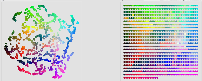
One of the (many) things I want to revisit is this idea of boiling down a corpus-specific(*) descriptor soup which will be then dimensionally reduced down to a 2d/3d plot, to hopefully then trigger using something like this:

API - ERAE Touch Walkthrough Series

Likely using the RGB LEDs to display a quantized UMAP projection:

At the time of this original thread we didn’t yet have fluid.grid~ which makes some of the translation stuff simple/trivial now, which is great, but I’m not up to date on whether or not the salience stuff was built into fluid.pca~ and/or if other new additions were added to facilitate that process.

So as a bit of a reminder to myself, and as context, I’ll outline what I’m aiming to do:

• take a corpus of samples (sliced “one shot” samples)
• analyze via the “grab all descriptors and stats” approach
• cook some of the data (loudness-weighted spectral moments, pitch-weighted confidence, etc…)
• use PCA to figure out the most salient components (say 90% coverage or whatever)
• use UMAP to reduce that down to a 2d/3d projection
• quantize the projection to a grid using fluid.grid~
• potentially apply some perceptual ordering/scaling to the results(?)
• use a kdtree to match the nearest point using XY(Z?) data from the controller
• potentially also retrieve loudness/melband data for loudness/spectral compensation(?)

Following that, here are the more concrete-ish questions I have.

(I know that “it depends” is the answer to everything, but just trying to work out best practice, and a generalizable approach that I can apply, before tweaking in detail)

Now, I remember a lot of lively discussion about normalizing, standardization, robust scaling, etc… I don’t know where that needs to happen in this process. Some things like loudness-weighted spectral moments, and confidence-weighted pitch would definitely go before PCA, but my gut tells me all of it should happen before then. That would potentially require a massive processing chain to treat each statistic of each descriptor differently. Similarly, I guess the output of UMAP may need to be normalized as well before being quantized. Is that right?

Is there a newer or streamlined way to do long processing chains? (e.g. getting loudness, pitch, mfccs, spectral shape, etc… along with all their descriptors into a single flattened buffer) Even just typing this out I’m having flashbacks of spending 2h+ trying to create a single processing chain that takes into consideration the weighting/scaling/etc…

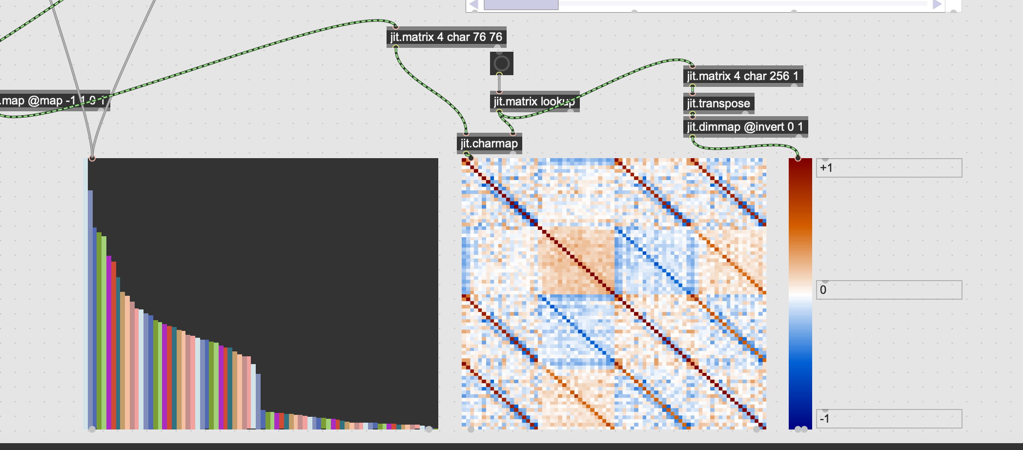
Is there a way of getting the ‘scree’ plot natively now? In the PCA/SVM thread (with @tedmoore and @weefuzzy’s help) there’s some hacky/janky jitter code that gives some results, but it’s not very elegant or robust.

Once you have the salience info, is there a newer or streamlined way to pluck out the desired statistics/descriptors post PCA and pre UMAP? I know that C++ versions of fluid.bufselect~ (and related objects) were created, but as far as I can tell it still requires a complex mesh of counting indices/channels and praying you have the right stuff in the flattened buffer in the end.

Has anything changed on the kdtree (rtree?) front? Like, is it possible to adjust queries and/or have columns that are retrievable but not searchable (like pulling up loudness/melband data, but not using those for the actual query). Before, I think I had a parallel coll, which is fine, but wondering if there’s a native approach for this “metadata”.

This last one is a bit more nebulous/philosophical, but as useful as it would be to map a bespoke UMAP projection onto that ERAE interface, I really really don’t like the idea of having to “learn” each mapping from scratch. I’d like to have some kind of indication or permanent correlation on the surface and the controller. Also considering that the surface is velocity sensitive, I’d like that to respond to the playing as well (so the louder I hit the surface, the louder that particular sample plays), hence not being sure if I should go with a 2d or 3d projection.

Ages ago I asked about somehow reorienting or re-remapping the UMAP projection using some perceptual descriptors (say centroid or loudness or pitch), without doing a CataRT-like, straight up, 2d plot. Or perhaps using color as a corollary dimension (red always = “bright” etc…).

Maybe some kind of crude clustering after the fact where nodes are created where top right is “bright and pitchy” and bottom left is “dark and noisy” and then cluster the UMAP to that or something?

So yeah, a more ramble-y question this last one, but the basic idea would be to best use the performance surface while not needing to learn each mapping individually.

*I have a more general desire to have a generalizable descriptor soup for matching across input and corpora, but for this purpose there’s no incoming audio to match

[tremblap]

@rodrigo.constanzo

Wow, crazy to think that this was almost a year ago that I was working on this stuff. (likely nothing to do with the job cuts that were announced in April 2021 at my job for which there are ongoing strikes to resolve!)

I’m so sorry about all this. I hope that your tradition of mammoth posts will help you take your mind off it.

I think that you know I appreciate your desire for rigour, but I’ve had so much fun with a more gaffa tape approach, with @balintlaczko for instance having after a few discussion devised a few descriptors he liked.

as for a stable perceptual space, I think that this is the most important part of it all, so I’d start with exploring that. the problem is that advanced timbral descriptor are not reducible to a single dimension (bright over there) so i’d use an approach that is much more perceptual. So that is much more my vibe with LPT - because we want control. The inherent maleability of extracted latent spaces is their streight but also their weakness for you in this context.

To start, I’d define what you care about (like @balintlaczko did) then I’d map those. It seems you come back to loudness, overall brightness, and pitchness. Maybe you could have another dimension, by pressure sensing of fader, on the shape of energy (could be volume of attack vs volume of sustain for instance) or the iterativeness (slice count per item to see)

===
another more cryptic approach could be to make a 3d space from high d, and then try to rotate it to fit a 3d space that you feel is consisten. The problem is that there are no way to make sure all bright stuff will be together, without thinking about how you do your machine listening…

so I hope you get more meat than the proverbial ‘it depends™’ but again it is very much in line with what you care about, which is very far from objective. That is the beauty of art, I reckon…

[rodrigo.constanzo]

@tremblap

I hope that your tradition of mammoth posts

Hehe, hopefully have a few more once I get my head back in gear.

@tremblap

I think that you know I appreciate your desire for rigour, but I’ve had so much fun with a more gaffa tape approach, with @balintlaczko for instance having after a few discussion devised a few descriptors he liked.

I tried this “gaffa” approach with the LTEp idea, but that lost all its momentum when I wanted to change a bit of the recipe based on @weefuzzy’s suggestion of using lower order MFCCs to reduce noise (which itself led to this thread). Having to rework the whole analysis pipeline to change one aspect of it was terrifying and I kind of stopped. That’s why I wanted to take a more rigorous approach as it’s not so easy to try “a bit of this and a bit of that”, since each one of those recipe bits takes me over an hour of really intense and fiddly coding to sort out (counting indices/channels and such). It’s the opposite of a ‘playful’ exploration.

Hence wanting to try the PCA->UMAP approach so what’s in there doesn’t matter so much (for this specific use case). I do like the idea of having a perceptually and philosophically meaningful descriptor space, but that may not always correspond with the most well represented space.

Either way I’d be baking in more descriptors, ala @balintlaczko, by including amount of onsets, time centroid, “timeness”, and potentially other bespoke descriptors.

Some of this does circle back to older concerns of how to search this data too. Like it would be great to search (or bias/reduce) by a custom descriptor (e.g. “timeness” > 0.6, onsets = 3, etc…) and then use a kdtree to find the nearest match from that subset (potentially not including “timeness” as one of its ingredients.

I did think of some kind of rotation or reorientation of the space afterwards. That wouldn’t be so bad as I could manually massage a mapping for each corpus and just have to do that once. That could prove to be impossible or problematic for reasons you’ve outlined (and more), but it’s a possibility.

Is there no known approach/best practice for further mapping/reorganizing a UMAP-ish projection? Or is it always meant to be “go explore the space with your mouse pointer” and see what is where!

[tedmoore]

@rodrigo.constanzo

Maybe some kind of crude clustering after the fact where nodes are created where top right is “bright and pitchy” and bottom left is “dark and noisy” and then cluster the UMAP to that or something?

As @tremblap and you said, this does sound like you’d be rotating and/or “flipping” the space to get certain descriptors roughly on certain axis. One approach might be to analytically find the “brightest” and “darkest” (or whatever) points in your dataset, then rotate the space so the relationship between those two is along the Y axis (for example). Then find the “noisiest” and “smoothest” points in your dataset (whatever that means) and further rotate or flip the dataset to make that relationship generally an X axis. There will likely be some tradeoffs no matter what (these dimensions may not, will likely not, be orthogonal!)

Instead of finding the “brightest” or whatever, you could try to find the “centroid” of brightness with something like a weighted average.

@rodrigo.constanzo

Now, I remember a lot of lively discussion about normalizing, standardization, robust scaling, etc… I don’t know where that needs to happen in this process. Some things like loudness-weighted spectral moments, and confidence-weighted pitch would definitely go before PCA, but my gut tells me all of it should happen before then. That would potentially require a massive processing chain to treat each statistic of each descriptor differently.

For what it’s worth, approaching something like this in the past, I’ve had success with doing a grab bag of analysis, like you describe, doing BufStats on all of it, Standardizing, then PCA (90% variance or so like you say), then UMAP.

@rodrigo.constanzo

I guess the output of UMAP may need to be normalized as well before being quantized. Is that right?

I’m not sure. I think I have been normalizing the output of UMAP before using Grid, but it will probably give you results nonetheless. They may be different though because normalizing the output of UMAP will stretch it somewhat–changing the distance relationship between points.

@rodrigo.constanzo

Is there a way of getting the ‘scree’ plot natively now?

A little bird whispered to me that the data for making this may become more readily available.

@rodrigo.constanzo

Once you have the salience info, is there a newer or streamlined way to pluck out the desired statistics/descriptors post PCA and pre UMAP?

I haven’t continued pursuing this idea (PCA/SVM thread). Also, @weefuzzy offered a bit of a lit review if it’s interesting to anyone. Since you’re generally interested in determining how these slices are different from / similar to each other using the principle components will get you farther than plucking the same number of original descriptors. Yeah, you’ll loose perceptually relevant axes but the rotation above may get you back to a good place.

Also for what it’s worth, since you’re interested in having the axes be perceptually relevant, you could try to 2D plotting on what you’re interested in (pitch and loudness or centroid and noisiness or whatever) then putting that in fluid.grid~ and seeing how performative and musical that feels?

@rodrigo.constanzo

Or perhaps using color as a corollary dimension (red always = “bright” etc…).

With whatever plot you have, you could totally just make the ERAE display color based on whatever analysis you want. (I know you know that).

@rodrigo.constanzo

Maybe some kind of crude clustering after the fact where nodes are created where top right is “bright and pitchy” and bottom left is “dark and noisy” and then cluster the UMAP to that or something?

Or you could do some clustering / sorting before the fact. Break up your corpus in subcorpora using fluid.datasetquery~ for a manual approach or fluid.kmeans~ for an unsupervised approach. Then run your analysis -------> grid pipeline on each subcorpora and then put the “subgrids” in a bigger grid, such as quadrants or whatever. You could even rotate the subgrids to try to get them lined up in some important way (I’m just riffing here now…)

[rodrigo.constanzo]

@tedmoore

As @tremblap and you said, this does sound like you’d be rotating and/or “flipping” the space to get certain descriptors roughly on certain axis. One approach might be to analytically find the “brightest” and “darkest” (or whatever) points in your dataset, then rotate the space so the relationship between those two is along the Y axis (for example). Then find the “noisiest” and “smoothest” points in your dataset (whatever that means) and further rotate or flip the dataset to make that relationship generally an X axis. There will likely be some tradeoffs no matter what (these dimensions may not, will likely not, be orthogonal!)

Yeah this is definitely a cool idea. Don’t know if this is a silly question, but is it possible to rotate a space based on a given criteria? (e.g. such that the highest mean of centroid is in the top right for example) Or perhaps give it multiple criteria and have it rotate to the most suitable orientation, then with some hand tuning after that perhaps.

The kmeans approach sounds tempting too, but I could see it being quite quantized in terms of the overall space. That may work well for combining multiple corpora and placing them in an larger macro space too.

@tedmoore

For what it’s worth, approaching something like this in the past, I’ve had success with doing a grab bag of analysis, like you describe, doing BufStats on all of it, Standardizing, then PCA (90% variance or so like you say), then UMAP.

Yup, that’s exactly what I’m trying to do. Though perhaps with more tweaked descriptors ahead of time (loudness-weighting etc…)

@tedmoore

I haven’t continued pursuing this idea (PCA/SVM thread). Also, @weefuzzy offered a bit of a lit review if it’s interesting to anyone. Since you’re generally interested in determining how these slices are different from / similar to each other using the principle components will get you farther than plucking the same number of original descriptors. Yeah, you’ll loose perceptually relevant axes but the rotation above may get you back to a good place.

This question was more pragmatic. As in, the PCA/SVM process spits out x amount of components which are most salient. This will likely be a list of arbitrary length and more than certainly be non-contiguous. So having a way to do that that isn’t a cascade of error prone single channel/single sample fluid.bufcompose~s from an unlabelled data container into another unlabelled one.

In effect a way to use the ‘scree plot’ to prune a dataset straight up.

[tedmoore]

@rodrigo.constanzo

a way to do that that isn’t a cascade of error prone single channel/single sample fluid.bufcompose~s from an unlabelled data container into another unlabelled one.

One way to get around this is to do some careful book-keeping just once. You could put into a dictionary what all the channels of a buffer (or dimensions of a dataset) are so that later you can just refer to that. Something like:

"centroid" -> 3
"loudness" -> 0
"pitch" -> 1
"pitchConf" -> 2
"flatness" -> 4
etc.

Maybe this isn’t what you’re referring to, but I’ve done something similar in the past and it has worked quite well. I haven’t really kept up with it, but I think there’s some potential there.

@rodrigo.constanzo

This question was more pragmatic. As in, the PCA/SVM process spits out x amount of components which are most salient. This will likely be a list of arbitrary length and more than certainly be non-contiguous.

If you’re UMAPing at the end of your chain, it isn’t really important to have the original descriptors after the PCA, you can just use the top whatever principal components (maybe that’s what you’re suggesting?). What I have been doing is looking at the scree plot, finding how many PCs I want to keep based on that, then re-running then FluidPCA and asking for how many I want to keep. It’s a bit of a double take, but eh.

One thing you could do is fitTransform into a new dataset (which now contains your order PCs as dimensions), figure out how many PCs you want to keep based on a scree, then just fluid.datasetquery~ to select the top however many dimensions (PCs) you want. I’m sure this would be faster.

@rodrigo.constanzo

Yeah this is definitely a cool idea. Don’t know if this is a silly question, but is it possible to rotate a space based on a given criteria? (e.g. such that the highest mean of centroid is in the top right for example) Or perhaps give it multiple criteria and have it rotate to the most suitable orientation,

I don’t know of an algorithm that gets at this… and I don’t think that the fluid-verse has a way to attack this. What it sounds like to me is to be able to “pin” a few data points in particular locations in a space (a 2D space for example) and then ask a dimension reduction algorithm such as UMAP to start it’s iterative shuffling of data points to try to optimise it’s cost function (but not letting it move the pinned points!). My guess is that something like this exists, but I don’t know what which algorithm.

[rodrigo.constanzo]

@tedmoore

One way to get around this is to do some careful book-keeping just once. You could put into a dictionary what all the channels of a buffer (or dimensions of a dataset) are so that later you can just refer to that.

Definitely. I started working out a thing like this ages ago to have a meta/macro dict to keep track of columns, as well as fit data and other metadata. And even suggested having some native way for the objects to output something similar, but it’s all very brittle and fragile if you want to change any single aspect of stuff (say, less MFCCs, different fft settings, larger analysis window, etc…).

@tedmoore

One thing you could do is fitTransform into a new dataset (which now contains your order PCs as dimensions), figure out how many PCs you want to keep based on a scree, then just fluid.datasetquery~ to select the top however many dimensions (PCs) you want. I’m sure this would be faster.

It’s been a bit since I do this in practice, but doesn’t the final step of the PCA/SVM-ish thing give you a list of indices (e.g. 4 6 18 21 22 30 48 61), then in order to build a fluid.dataset~ from that (to feed UMAP) you need to go and fetch those individual columns. I guess there’s perhaps some zl-land munging that can happen there, and since it doesn’t really matter what these columns represent anymore, they could be moved without labels or whatever.

It just seems like a useful process that would benefit from some kind of native-ish solution like telling fluid.umap~:
weights pca.output 90(%), fittransform source.dataset target.dataset

@tedmoore

What I have been doing is looking at the scree plot, finding how many PCs I want to keep based on that, then re-running then FluidPCA and asking for how many I want to keep. It’s a bit of a double take, but eh.

Hmm. I could be remembering wrong, but doesn’t PCA return the same results no matter how many components you ask for? Like the first 5 components of a PCA5 are the same as a PCA500. And that the dump output of PCA contains the whole matrix either way.

@tedmoore

I don’t know of an algorithm that gets at this… and I don’t think that the fluid-verse has a way to attack this. What it sounds like to me is to be able to “pin” a few data points in particular locations in a space (a 2D space for example) and then ask a dimension reduction algorithm such as UMAP to start it’s iterative shuffling of data points to try to optimise it’s cost function (but not letting it move the pinned points!). My guess is that something like this exists, but I don’t know what which algorithm.

Yeah that’s interesting. Again, doable by poking and vibing it, it just gets tricky if you’re trying to orient towards a position that satisfies more than one criteria. Or using that as a jumping off point.

[tedmoore]

@rodrigo.constanzo

It’s been a bit since I do this in practice, but doesn’t the final step of the PCA/SVM-ish thing give you a list of indices (e.g. 4 6 18 21 22 30 48 61),

This is true, however I think since you’re planning

@rodrigo.constanzo

(to feed UMAP)

there’s no need to retrieve the original descriptor dimensions at this point in the pipeline. Both PCA and UMAP return dimensions that are abstractions / distortions of the original data (projections, or embeddings is the word actually) and since UMAP is at the end of the pipeline you end up with an embedding anyway.

If you decide to feed UMAP a dataset with n dimensions, the n Principal Components will always (!?) be better for UMAP to consume than n of the original dimensions, even if those dimensions are selected in some clever way such as the PCA/SVM thing.

I think the benefit to the PCA/SVM thing is only if you don’t have UMAP (or some other dimensionality reduction algorithm) at the end of the pipeline–and you really want to end up with some number of the original descriptors, but are curious about which descriptors might be more useful for representing the differences (variance) in the original data points. This could be useful from a “know your data” perspective.

====================

@rodrigo.constanzo

I could be remembering wrong, but doesn’t PCA return the same results no matter how many components you ask for? Like the first 5 components of a PCA5 are the same as a PCA500. And that the dump output of PCA contains the whole matrix either way.

This is correct. If you fittransform with PCA the output dataset will be the n principal components you ask for. PCA asking for 500 will give you an output dataset with 500 columns, PCA 5 will give you an output dataset with 5 columns–in both the first 5 columns will be identical.

@rodrigo.constanzo

even suggested having some native way for the objects to output something similar,

This would be cool. I think with enough people kicking around this idea something interesting could surface. Not sure what that would look like at this point yet.

[rodrigo.constanzo]

@tedmoore

there’s no need to retrieve the original descriptor dimensions at this point in the pipeline. Both PCA and UMAP return dimensions that are abstractions / distortions of the original data (projections, or embeddings is the word actually) and since UMAP is at the end of the pipeline you end up with an embedding anyway.

Hmm, I could have grossly misunderstood what your PCA->UMAP processing chain looked like.

I was assuming(/thinking) that you would PCA only as a method to determine which of the original dimensions to then pass along to UMAP. So the output of PCA would never be touched or used, other than to compute the scree/salience info.

So PCA would be fed loudness/centroid/mfccs/mel/means/std/pitch/etc…, and then spit out “gibberish”. Then UMAP would be fed loudness/mfcc/std/etc… as a subset of the original larder dataset.

Hence the conern/worry of having to fish out all those individual dimensions in their original(ish) places.

@tedmoore

This would be cool. I think with enough people kicking around this idea something interesting could surface. Not sure what that would look like at this point yet.

This is quite a niche use case, as cool as it is, though the ability to go fishing inside a dataset without having to get knee deep in SQL-land would be fantastic. Even to copy out a single point from one dataset to another using fluid.datasetquery~ would take me a bit of squinting at the help doc, and print/dump-ing the output to make sure it’s correct. It could just be me, but I find the syntax super unintuitive.

[jamesbradbury]

@rodrigo.constanzo

I was assuming(/thinking) that you would PCA only as a method to determine which of the original dimensions to then pass along to UMAP. So the output of PCA would never be touched or used, other than to compute the scree/salience info.

I wouldn’t be too stressed about the latter approach. Have you tried UMAP-ing the PCA values and seeing how it sounds perceptually? You can also, as a note of interest, just look at the number which pca gives you (the amount of variance retained) as an eyeball. I’ve had stellar results with this keeping 97 of the variance which in many cases has done things like take 240 values to 80 for example. I know that is what AudioStellar do.

[tedmoore]

@rodrigo.constanzo

So PCA would be fed loudness/centroid/mfccs/mel/means/std/pitch/etc…, and then spit out “gibberish”. Then UMAP would be fed loudness/mfcc/std/etc… as a subset of the original larder dataset.

Hence the conern/worry of having to fish out all those individual dimensions in their original(ish) places.

I see. You are now correct that this is not what I was doing. It is the “gibberish” (aka. principal components) that I fed into the UMAP. There are three benefits to using PCA before UMAP as I see it:

1. You can end up with fewer dimensions that are actually fed to UMAP making the UMAP computation time shorter, without loosing too much important data (or at least knowing how much variance is being lost)
2. PCA can remove redundancy in the data so if there are a few original dimensions that are basically redundant PCA can sort of “tell you that” and give you data (principal components) that “avoids” that.
3. PCA can remove noise in the data, so if there’s a few dimensions that just seem random across the data points and don’t have much or any use in distinguishing the points from one another (which is basically the activity we’re after) the principal components it provides back will also kind of “avoid” that part of the dataset.

The last two points being useful in that it can kind of focus the data on what’s relevant or salient (i.e., principal) so that when UMAP constructs it’s initial distance tree (part of it’s algorithm) it’s not considering (as much) noise or redundancy when trying to compare these points to each other.

[rodrigo.constanzo]

Interesting.

I was thinking something completely different.

I guess this is something test-able, but I would just assume that since PCA tends to linearize and not handle certain types of dimensional relationships (orthogonal) that it’s use here was just to prune back the “real” data to what is likely to be more important. And then using a “better” algorithm (UMAP in this case) to actually make sense of the original descriptor data.

With this assumption, wouldn’t all of the points still be true? In that you’re passing along data that still meets that criteria (less dimensions, less redundancy, less noise) but in its non-transformed state, potentially to an algorithm that can better make sense of non-linearities etc…

[tedmoore]

@rodrigo.constanzo

to prune back the “real” data to what is likely to be more important. And then using a “better” algorithm (UMAP in this case) to actually make sense of the original descriptor data.

exactly.

@rodrigo.constanzo

With this assumption, wouldn’t all of the points still be true? In that you’re passing along data that still meets that criteria (less dimensions, less redundancy, less noise) but in its non-transformed state, potentially to an algorithm that can better make sense of non-linearities etc…

totally, all those points still are true. And also true is that…

@tedmoore

If you decide to feed UMAP a dataset with n dimensions, the n Principal Components will always (!?) be better for UMAP to consume than n of the original dimensions, even if those dimensions are selected in some clever way such as the PCA/SVM thing.

======================

When I do the PCA → UMAP thing its’ generally because I am starting from hundreds or at least dozens of dimensions (just throwin’ all the analysis at it). If I only had a dozen dimensions or so (13 MFCCs for example), I probably wouldn’t PCA first. Maybe interesting to check the scree plot but I wouldn’t consider it necessary.

[rodrigo.constanzo]

@tedmoore

If you decide to feed UMAP a dataset with n dimensions, the n Principal Components will always (!?) be better for UMAP to consume than n of the original dimensions, even if those dimensions are selected in some clever way such as the PCA/SVM thing.

I missed the last bit of this on my first read/response. I thought you meant that the bits selected by PCA would be the best.

Is this from your experience/testing or is this like one of those “known” things? On first blush it seems super counterintuitive to me (like transcoding video files).

[tedmoore]

@tedmoore

If you decide to feed UMAP a dataset with n dimensions, the n Principal Components will always (!?) be better for UMAP to consume than n of the original dimensions, even if those dimensions are selected in some clever way such as the PCA/SVM thing.

PCA essentially “rotates” the data to maximise the variance and then reports back the new dimensions in order of how much of the variance they explain. These new dimensions are called the principal components. If you’re looking to have a smaller number of dimensions, you don’t want to be throwing out dimensions that have a lot of “explaining power” (meaning that they help you or an algorithm understand the salient differences between the data points). This is why PCA reports the PCs back in order, so you can take the top n PCs knowing that those will be the most “useful”.

And by useful what I mean is “able to reveal the salient differences between the data points”, which is the kind of information we want to give to UMAP because that’s what it’s going to base it’s embedding on–the differences (i.e., distances) it calculates between the data points.

This is a result of the algorithm, so maybe that’s what you mean by known thing. It’s not an empirical conclusion. It’s a mathematical one.

It’s important to note that PCA only does linear rotations, so if the data is very blobby this is fine. If the data has curly manifolds to it then PCA might not be good because it has to way of untangling them. (UMAP and other iterative based dimensionality reduction algorithms do try to do this untangling.)

With all of that said, if there are dozens or more of dimensions using PCA first (and taking only the top so many PCs) can rotate the data in a way that can reduce redundancy and noise in the data set (a curvy manifold will likely be lost by the process?), while also reducing the amount of computation UMAP will ultimately have to do.

Hmm. That’s a long answer. Longer than I thought I was gonna type. I’m not sure if it got at your question? Let me know!