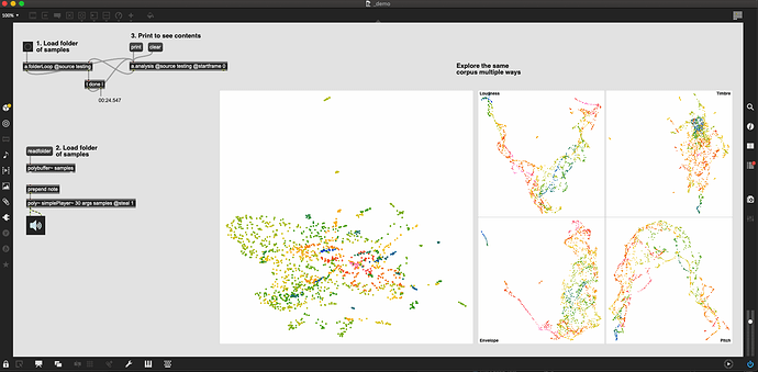
After spending a few days building the first step of the LTEp idea, I wanted to share some code showing where it’s at.
LTEp(2).zip (80.7 KB)
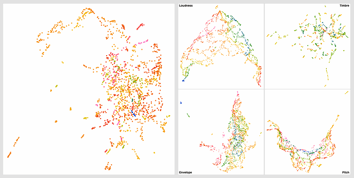
You point it to a folder of samples (individual samples, no segmentation here) and let it run. Once it’s done it will plot the composite space, along with each individual sub-space.
Each individual subspace is as follows:
- Loudness (4D) - mean, std, min, max → robust scale
- Timbre (4D) - loudness-weighted 20(19)mfccs, mean, std, min, max → standardize → 4D UMAP → robust scale
- Envelope (4D) - deriv of loudness mean, deriv of loudness std, deriv of loudness-weighted centroid mean, deriv of loudness-weighted rolloff mean → robust scale
- Pitch (2D) - confidence-weighted median, raw confidence → robust scale
There’s still some improvements to do all over the place, not the least of which is optimizing the scaling and things like that, but for now everything is robust scaled at the end, and prior to that, each subspace is massaged a bit to weigh the internal components (e.g. I divide the pitch output by 127 so that confidence matters a lot more, and I scale the deriv of loudness up so it is more in the range of the spectral derivatives).
The visualizers are a second layer abstraction as most of those are 4D spaces that are then getting further reduced to 3D for visualization. The Timbre space in particular does back-to-back UMAP-ing to go down to 4D then down to 3D again after that. The Pitch space is also dimensionality increased to go from 2D up to 3D. I’ve also plotted the raw 2D version and you get more a vanilla x/y looking plot, rather than this banana, but the overall mapping and direction are similar.
It’s interesting to see how effect the spaces are organized internally, and then comparing that to the more complex 14D space that makes up the composite/overall space.
Oh, I almost forgot to mention. All of this is computed on only 256 samples. That should not come as a surprise to everyone as I don’t shut up about it, but what’s significant here is how differentiated things are even in that small time frame (for the audio I’m feeding it at least).
The main analysis abstraction can be fairly easily repurpose-able for real-time matching, which will be one of the next steps. As I think that will yield interesting results.
I also plan on analyzing multiple timeframes on each pass, so I have 256 and 4410 sample windows, along with “the whole file” as well, to then incorporate prediction, and hopefully weighting in the future.


