Edge cases in analysis frames

[rodrigo.constanzo]

Revisiting a pretty old subject here, but in searching on the forum, it doesn’t look like any of it took place on here.

Back at the second plenary there was a bunch of discussion between @tremblap, @a.harker, @weefuzzy, and myself about what to do when you’re analyzing a small number of samples and want the best representation of what’s in there.

As a point of reference, I’m talking about analyses like these:
@windowsize 256 @hopsize 64 @numframes 256

So in a situation like this, you are returned with only 7 analysis frames. So taking the vanilla mean from fluid.bufstats~ probably isn’t enough to remove the impact of the edge cases here, particularly since the only option here is zero-padding.

The intended use case here is that I’m trying to shorten the ‘onset descriptors’ analysis window down to 256 samples instead of 512, since I’m now doing some extra analysis stuff, and further post-processing. At the best of times my latency here is ca. 11ms, but now it’s getting closer to 15ms+, which starts feeling laggy.

From my vague recollection, what is “best” (generally speaking) varies on the type of descriptor in question.

For centroid, I believe mirroring (vs zero-padding) can be better because it keeps the spectral emphasis more-or-less in the same place (though that’s not possible here). For something like pitch, throwing out the outer frames is desirable(?) since you don’t know what is in there. For loudness doing something similar to avoid overly weighing the “zeroes” that surround the analysis window.

Is this about right?

I’m not sure why this is the case, but in my patches from around the second plenary (which I’ve just tweaked as we’ve carried on) I’ve been keeping the first 7 frames loudness (although from 512 samples, so 7 out of 11 frames), and frames 3-8 for spectral moments (again, out of 11).

So that doesn’t really line up with my memory of stuff (hence this thread, and generally inquiry). The spectral moments “middle frames” makes sense, but not sure why I would only take the first frames of loudness. I guess to try to capture the initial “oomph” of the sound only? With only 256 samples it’d be all “oomph” I suppose.

Do MFCCs and mel-bands fall into the spectral descriptors thing, where it would (perhaps) be better to grab the central frames?

////////////////////////////////////////////////////////////////////////////////////////////////////////////////

Another thing that occurred to me is that I may want different amount of frames for different statistics. Maybe for the mean it would be good to be more selective about the frames to not overly weigh it towards the zero-padding, but perhaps I do want the zero-padding-ness for the derivative, since that may capture more of what the actual morphology of the analyzed segment was?

I guess I can always ‘double dip’ the fluid.bufstats~-ing by taking some stats from the whole window, and other stats from just the middle etc…

[tremblap]

@rodrigo.constanzo

Is this about right?

I’ve found that on small windows it is so signal dependant that I have to test. Sorry for the ‘it depends’ answer but that is the most truthful. The best way to test I found is to test values with expectations. If I do something pitchy, and something noisy, what do i get value-wise. Some of these examples are in the Max helpfiles as demo (for instance bufpitch granulator on confidence).

[rodrigo.constanzo]

So far, in comparing the results from the 512 version and the 256 version (doing frames 3-6 instead of 3-8 for spectral descriptors) appears to be about the same.

Am I correct in assuming that for all the spectral descriptors, with such short windows, that throwing out the outer frames will be better, since you otherwise risk pulling the stats down towards zero(padding)?

The statistics (derivative/deviation) tend to be pretty wildly different, but that doesn’t seem far fetched to me since it’s a different and shorter time-frame at play.

It doesn’t hurt that with loudness I was only doing the first 7 frames before (@512) and now I’m analyzing all 7 frames (@256).

So I guess the overall thinking is focusing on the frames you think will be important and testing from there?

[tremblap]

@rodrigo.constanzo

So I guess the overall thinking is focusing on the frames you think will be important and testing from there?

indeed. For instance: I’m editing right now in Premiere and even there, super high level, you have the option for blurring on what to do with the edge cases (mirror or zero-pad - although the latter is not explained…)

[rodrigo.constanzo]

I was about to make a new post, but discourse suggested this one and it was right!

So I built a patch to test some of this today.

For context, I’m working on the onset descriptors idea where I have a 256 sample analysis window which I’m running with @fftsettings 256 64 512. This gives me 7 frames of analysis, which I was then feeding frames 3-6 (@startframe 3 @numframes 3) into fluid.bufstats~, to avoid having the zero-padding on the edges muck about the spectral descriptors.

Since there’s no option to select what happens with edge cases in the fluid.verse~, I’ve “manually” mirrored the edges using fluid.bufcompose~. It’s a bit ugly and a bit slow, but it (appears to) work.

The patch below compares the original version of looking at only the middle 3 frames, with the version which mirrors the outer frames and then analyzes “all” 7 frames.

Don’t really know how to properly assess how effective this is, so I built a thing where you can manually listen to each fragment and compare the results using an sfv~ filter.

----------begin_max5_patcher----------
7231.3oc6ck9iaibk+y1+UPnr.KvtsEp6ic+xjIGd.x3IyF6fAASBZPIwtMs
USpPQ018DD+29VEKJJRwqhREoTOy3.zCCOT8pe06pd0qp2+5kuX1h3OGrcl2
+i2O58hW7ud4KdQ1sz23E4++ewrG7+7x09aydsYKie3gfnzY2XdVZvmSytOc
t2hv68VEd2cAIAQKC7tKNwac7m7tKI3etScmPUCk+UqCiBVFuKJ6Sw42bSRv
V0ureZXbzsUdCZ9abWbT51veJPeODXNX+G5mt78gQ2eaRvxTSeAKmSuwCJ4y
gxR+CiT2jQUeoGiMG38OJ8CG4+P1O7ruIX8iAogK82SsQ6dHLZcPZF..K8I2
4uLn78TuX7tz8u4dxKbU1Oa7hO7JHhNSey+8Keo9O2XIl+Pv1s92GTCywHNa
Vuf.CLmWFDD3a7vYX.BUBCpzKQM1ifM0iv6o.yKl9zl.SyOal2+3D5rswfwl
6El9et0yWwmk5sUwYMe97FYnP8xPgGNCEPNGT5ePHQghX7bLEQARDDHHTIVn
vanTisjKC+EXlCgbzh4JI33O54mpv9YCFzjP8i8vBwbljSjHECK.HATMLgLr
fWDXBJGeXpctOzoBjbz0FNJbINRl6sYs+SdJfa25zsmnr8vQWHWifTEFiP7p
ByJN2KlrLj+yAvkIH0UbRoWaXMykXMdtm5Qa7SBNS3lbB1oZ.tU.cUW.nZ+B
x9gtT3M0oJf8UJfC2lFD4kFWRE7Yx5REYVxgDbcGnjWRlUhKAO3buzjv6uOH
wKwOZU7Cd9Q9qeZa31Iy4JdlILHJ6ub3EDYwtDYAZ2B7WsvO59g66DkAxsqS
Ky6IIERtWHS9HWNClso9IocLEFRFmAkgpat.ib0TX.LGOElnfOo9gq0Y01e+
hWTb31fd6xLkd7ZSsfC5tK27nHpotLu0t71v6Ux+ytwaVFiqKAfsOd2W7D.k
bAXNseHPoCfvOZTmK5FBvMBAjlf.gEPPGW4Rf4+5KJDQzAhnchRgH5IRANho
f.blbfrOD4j5yA+zJ+keo2NGGqbR4XgbCmf9uCoy0ndKfK0acrd8lXhk75dh
gD0UmSENZ.TJlF8XouObaVGNHYn8eFod+mwcjVMIs89+MYXP9i25+39G7a9N
8ipzi7l8+p+yu4+S+2fnUl6bR.3oZ1igYiucOwUkYu7t73Z2iKulM6sGBFU6
d7mSl8XlYFLt183nKiYu7N23Z2iCm4twq+aO5bAfHExN5VbQ1D3ZbYGXRGMl
QgsNlcmx1b5oMjsXWZZbTWCYRSeiRp22PYdwn+6PTRAKZrD0r2RCRtMHxew5
fVFNofV62NWs0F+kezKyRkRJ0ip0eYwveNDg.z5PjF25b7mX63OYhb0Yq+Ca
1lF+v1tDj4HbFWAjMuhuMbjR51UN2PPVn29L386WckYfECo0WSUmotBKm4ZG
Od0qdUbz1fCwfsClVkNqZ8MgvQifXwkv4iMdO3Gsye85mdSXRRbhpi+GVceP
WnAJWLkZBHGwY..uakWG59koMkK4lNcdu9EytKbcviAIaCU5pOz9uXl+lMkt
8KJ8IZn5CwY+PhaJtUXj4VvhakD7X39umVbW+DEBkpfmcIl3q8YFY1gel3UA
IQ6By9kL2TMnkSRYCO53xoldgIRaYih6ebov8YB0LvLUXSfmIxRBTpg+6WGu
7iAqJI5nPxMAQgQkCFakGuJ3N+cqSusbbGyhyZCOeer.a7gEwV72lDp4Tyek
6SBWEGoIhJiD5auu49QkZeiQyxclr2HxeSCerhUQAKs7Pk8nzcaW3mnGnxsS
h1+vz330UeTw2sN3tz7GuILJ5HTLMdS6OLI7922w2tHV8vG552N6IaucWj4o
2p3IRuc+bPO7dJYzbY3p+7e1OJ7A+zfzvGxiabwCM9J79sKShWutR+07jGa3
IqT73KC9T3pz2m0PkYFTud3l8LQyJFkWEpTXjV8do92us5c1l9jAzKcqcKxk
guMM3Ak93zidAkzQ31zsuO9S6m+8dFsx.vgLTprLcYEhUteWJFOJRFdKN9+U
98ZZshAYVJDLyZUvlygDjfl+WDpphxVUV1fBSYomT0A9ROnaEmm5+0Xu4E6s
4jqB6Dg6pw7ng3dbm1SWkqddp9e10aUnhmh4KszigJjrT.1Zc4NwYFmvpoRI
3XJWYwFSEHHlpi0F9XCWs5YR6dcVa7.z43wEAKo8fkP6vRyxJogTrjvHRBlg
gBBgowRzHfkL40GVx5AKA1gkfLEDX0jljPk1AIkHATBmxFK9RF+5CKQcik1A
kHgYJTL7bECox0HFCxkP.iqtImMFPI65CJg8vVZGTZVacDhNWR4BpjyITDGy
EiFTRu9fRP2PocFdPTiG.pYGRT7jHoPvUrnLgbzfR7UNTxqAkX6fRrYtOTCy
4n.dzoT6XGNbd25cgqluX2c57CKdavW79psw6RVFnCSw1MJLIwe8126uIv6q
zfYXT1b5p8zaeHax7de0B8bBU3oGxNTlnj8Ku9JBjdEHgx9w718bE2LlSnV4
4pIlU235AgLB2Nm4Q41p2+21w.vP46vj9wfJM29bIp7rjx9MiVE74RgXvIXj
gd5AjLqyRi7M1.Ysy1.ZAxpv1b8gG4LMSHfvFDffZ.PND2Ecl50xroy5q5m2
LRYzSky3telod7JczRprJ8hZkud.KktOIpfYAUnseNtTA0FpfN1TAwFpfM1T
A1FpXz4KP1PExwlJfVPE5vJLdTQ9OduTAYL4N2CzWXpfeUPErqBpfdUPE3qA
pfdUvWn8WzJpHSwxnp0RXAUfGcqY1fE31slkey8KHWVl+s5VyJLcqeZZR3hc
oFGhJuBiCZkPtec7B+0Gs7EMsPIu7.w4l010hrPEBQYQtk1vVvjdRKraCYiA
FNBYkRa4N4hvMwq8Szwd3weJN9A8JXo9mzBP.BZZCTRvNJojvnIZqP+v9Ux+
Fyd04mzA.ve8Zu+9rj.+0+8YdlPxblaxullLHRuWnfRNaeNtnSfWJngsAMxj
tH3gwc0TNg3z8zbTrWI3KNZ8Skvv+9L8Jzln.PhUPXCrZDdC.DiXhvEvQPB5
zRSlcOrnyT1FyE0IdcNITIoXzg3befjOsbBwxjcCw6LetGgTkYwN8oWQW4FC
Qmzl0xpenR.nRlewU1O6IWGAVOXSl8K77ggkGCJA3WyGleMeX907gYzxGFsC
kZ+t7f8tRhY7vXZluS02eFCIrmsD5bz0wJ1jsuU9RevgYATxgCBYDfCQ2K+W
kcpv3iJptdbxpp6pm9.GY153aShjfGL3.ul.GiWD4fiR8TO3CkVBdjzyg2A0
B7zcNKUrBbtOYvr.kZYoMuUaYaq2WkkA9J2p838.i4aiPVk8OFCxxxDLxHfp
nmUn5fgy7r8G2.bRXiAbhttgSylHv6CwQ2u9o49g2YE+nIFKvQAwf+hQpFxq
JUCnvwRpV9LDUKvSrs3IRLGxgLAFgP.o.IoE62CGimD9Oq0Rlu8tvMvdNJx7
BxyH3bOPxsDGk58WnjRITA.iXLtNaYA7wfq7rscOJoTgv1kBSLlK+C57IhCn
S1rfaAdNDDkcqBieaVnLt8MAQ6NL3rOnKMS5Kt+tv0qWFuNNozKT5MTLo4ip
yLu0MkdTw28ipY8ijDHTn5OyU97vQrrqTWjcToUFLx+N39OjnSsaj90ILDmP
ytRfTyETeEngOEcnMAPookTJgADyUpaoTe.O9SUbh4g2geHFE4QxOdSbRQrt
likU9tcow2m3uJLOqg.EOqX75P.5LAmU8l0CdgVefZfHr7uQSbaECpe6thCf
pdGH8WtT0nUFPvHEvlgHDkhUyHC2buivlYAqCd33OmKT5OxFLD.nPXtR8Ko2
hNG+8kCnmh29OuIHx6s9Qa8davCgKhWu53bzqT6P3zrcahdzDKjlqnP.qA5b
qhPWpGmpRoH0Km0+fLNxv0H..cfkO9GPqwM6auMLRGZ2fBNIrxzCyz16YGQb
AAWmSZPBMELNcH2L.d3pRNhB4EAGPEByUMRzGK4v1yRvz+iatx7qMIBNUfyJ
3gDPf7L9VEy.gyM7cHogWjxJqtbDD5dieZpsBckCBtNuFaPpXeLv+QsNvQkv
+9ea5sY+LfSj7O1AgFToXOWywpDLQ4ucs.Rp19gYDlvAYxCZwAbCZAVtNvOo
zWmMQa0Og9LewPcJwANd.R+Ye+9+7yQw8A8oSs7toy2zUYj1nJ07Cu6OdhhK
h9EWn.NKa.FvnXXl3BDhfHKs.SXPHv3NjDwHYLMTITn2sQ8Ht8MOsJI99fn2
kwX1pTGT6olQupVTKypGeuOaG0BENAWkcV6rWlIWUGixL9an4vx9sjWmBR16
YzUmCmsKGAYXklyrQBNgIk4WAjSgXT1rbCWdZhRx9kjH4lBZ5pdDEdcPTvi9
c4.5.9sOMKHMK53LiNsLwrC1MvRtQiOVlajUeKJ1sr6U5bhB+oqe0YInXkrP
e83oPV3qKeVX0qDQc2YDEXOH+pIiz+8kxHimUD9q8Ci9xIP4JFqB6e0uZ5H+
seJToo3jmyOLWSxg+LozM5YGg+m1tNbUPhszciNoM.qG8zi6MPGCosNRiXci
MSA99sAqNGrk0kEx5Jdl7t2a7SSB+7xzjyPa4zSz57F8KSEK+QrgWEpY+t3U
E4k7Y5ppC0HXgOSSB3LLUhWAJY9txYkcuDbSZVq63xDR9ee3xzIvLzjzUzYM
b5yROGe6x3MAmlqiGV0JIV+uVmQ202.167WbNLcCXRdytB67p4xuXPSRqg.S
.FhKJW.ObeW7854VeFCxXNivgFC0DLLKF.jZqL6U3ro9qOLfEB+JXn5G7eL3
t3jGFoIvdVyt.LmNxfvJ+jO9pH8Ni3UYgK6LjIGxZIUDPuSXkRZItdjBcg7h
URtXMkEYzwHDVbXOxqiVj9FsPhOUoYwGx2nH.PoLWbL94Qm5bNnctxpKVGnr
gYx2huNN9iy5bwR6b0O.VwfeXUfqcw3EDa6o5ek0tDuWXzGOCMoLUeEHJbwA
y.JMgVnD0xuqwX9X2mdReSMQgCq+Y1mfKekcFMsroaSP5lJ+cDVDngQmW.aI
S6hj1q08QUb7il44+C5M+6yAGSWqcGaXSQpQQ5BuenEZr2yY0W7BARRdJAJk
XAO+JtXRln3C9elUZ2UeBJPEUmbLOWdvUIlT6LGiuC6Zv4nyHxgDzDDlhjUs
hqEMgS03ZsCn0tI9KYpiUJAv1m0c0upGcxbgNipuowqtPNA4xbrttj5v4HN9
vqbnA9tTdrOYgxxrmR9506BJuY1FdphC444NzAc0xxZnmhNQR7mhNqdQu1Yl
fdwu6I+yqS.PRpIU+3bLFYjwQPkmpSWm30IAAmYuHaTnHb3Pl1wqoqC7Fkl8
nT+ypKHH.FyDLeFP0AxFRXRnjNc8i+RvpypOvK7ZGVLqYPtk2opO72BVuN9S
12MpmU5TI.H5KCAEHpICa4BnHaJKpuiRnSdGE8y4NZ1Rs9530mIaYQXYoJOi
oljVcxR46M6R1r97c7iWjs5DHUoeKSQsVMG0hY0P.FmeQT.SlIfhDTFRLE8+
jfkAgOZeFPzDOXwjmOz2Ak2HHiaGvLMZMa3I4sFinTrKyMrxy2gQT8wtWuib
WVN2sAQq19bzp7gArwUuQq6tH.GB3lknmv.x78TFGNI7qo9aFhMgRw1+a8Si
89VcTXlM5z31zf61sdc5fVv3pnLAB4YCOrh4LpC6XS6Wki27BBJEZVpLFliM
aDSlRkBaZFfLc9zydwxGRntbE1gDbgwQUbgnMFIwxIwZRp9fb6439k7S5nv9
zoQ555LeWqI2uOLI8Iu+v8wyrXID.5Q9r.xfyGvUZ5xWBaqCT3.1YlMuVDPo
DXljiRpijmEVL..Cy2HWm+fwOSNKoy5YUxXuFOJXY74nZmis.R8C5Wr4Dkg.
56rfUe7IsGp697gU8lpuWQ0kr7CQ7RMfkmfrP.nyiP1S7jo1NDDQZ3j.94FB
JkiA.1xQ6stz5ffJk+jtNAdgTKwUARaRQR2ez7psm4fi4aIeZp872klc3l2A
TPo34ziOLhojFNMtITGcTuKlnNepGXncb0zhlK.pYlJfXhNIpD4UiW2zwau5
sGFk51yg5ffO1yIn1fYJTRVPFBQnHAVRD5cHMBzC1fsFaZWIg4jTxohE6Kgd
Y.Q6EPuCmMZYmoW8cfzUppE58UkJpgkKwdYOPo0O7wCmPtUOY3wCkmEPavd.
lZJ+6CioE2fpJP2ElgFJ+dNRUtPLWJDhtTjiv5hiqRyMKGQzqd5TpHWftVTj
CMGmxiqpaD7ZP0cdWcbUVivWZk08okd+HdC5kgLhizKKwWg5kaUgbOZhwmnl
3VKyI39YRaT6rd3old7yWWMhN15pOmpHDMimDyYywYcZJlKnDodh1NqLBAEW
6kQHCJPPf5nf6JiPPW6hcaPfZRhlSty1bN5FuBTZ14T0fjPPq3FBScEtgcLt
8gs6Bm0euRYICBNRIACaxkMA9P1u2rTgt3sTDnmBcnOFF7o4env.Ry8caCBB
8hyO0DiTq.ZyUoKovQrIxKBWhxO24zqK9BBywHQkTssQO9M0GCj4uj8+8TLa
XYejOBVTZwLZhezJkYDnVAW+XfxIBZ4JFkdUzELGwhSbu2usJyevas+C0z25
wOh7NeikTLHzY0guIZZcEN7VVUWEGeyqY.e0cA95hk01FbF9t6RUuSpBm1pf
GlhwviBQkc7Ue2Rt9Nz3NrGyI5J2WYLGqKuCvQwWVLdr8kU84JpnSVMiGqjF
bgmVqdEMSuyU8y9T1nUO63rQpd10uhWtw5YS0otoQOLY5TDuwa4lc5hCVwpy
zb0dqKtF0zxqw0vnMv0zRkf6D0bw5c95+BrR.hLkKOSgiBZJSRHLeTJEfPkU
YJTvJjP90BC3uVX.+kRgA73cPRyKqsoT1xMNqQ2+2So1b.rnrFsuL9penx40
fjG8W6EF48vVuvsdIA5MkSvJOEdToLzEFsJ3ykz6L5U.kpULQqzozVTlLE7j
bK1FscfNxWmpJZdwHW2Emz5JixN9RshcGCs4UUVJaxwVrEUcloBbe0gkj5rA
1bkBlPfhQyomGthFJtRthvUGpJfHtnZBn+7US.gq4QubJBXSMC6Qa04tTOR3
1ZZGLztM2FNpVr9qep2VkCna8TN3oCEhezpbO.TNCj6aPiNAflXfzH2Nh3n3
7wQeMpkCjcBdvIq3mYYYGiNhk9Ltkz.ZDoAlkzfxnW0rL2gz.0RZfMh3.wRZ
XLKEd3ALVboKGe3NpFeielqaWXTNi7aOCAppuwDjviwy7PEVCGgnJilsMRVA
tmEmrxDlMPiAnzssMt4lFdVMszlVFBDyJUmCcUaC04SQ+MNDLFc7gz3PmOfC
XVA67CBsmQaoG7P81VRmzVbqYmN21RJrnojTGzRba3T3tnOwsYnhibPKIrtO
4blegM79bWvNxQ1zRvwnSZeS6bMaTfMFxbA6JwFQPrSZITkAoN5SN2JEEZKb
hlhNIENFdff3Cv4mypkvVwyHGCYR6aZmKSxI1zztvbOFOYsjM7LLW0PPKZHm
K6aUKinMywfF+lVBFCkAXarcQbxHqM5VwtPsizFihhpJHrn7ub555sfbNRor
qb+xNWzGkIcgrY7VJGEKb1zzBzXnE4HEDsLXimLdOqh1fD6hYYXCuljOJyxv
Fi8B4TMUpiPhpGOJBJEyoHgTByqss.fDI4XNPBAr75ui5ob.W.fBnPT8nuXR
iFzQRRiVW4LCwhMi+PmDfEqTn5h.Q.wSUKImJO.rZdGtXBjWp.rZk63tPWqU
QUo9PlIv4GkBn513nT+7nz9rdJe1d5ddbpdlsRCl7b6nf0eXA02sJL9sYIo3
suonRGczoXTNRzv4P890nn4BHvwGAzDHzTxMzELAygA89xD+gkxr5gUcoiC4
hCceh9.mFWshcbhEOflOpoa+XltkiX58qPxMur8yynpmkQkY7JFL91cK86Z.
noybYqJB8MdJiwELF2TEC.FqC5iyNJ.UsVOc7oR0edSPdYh4sAODtPe7I1rI
JBmBw4m59XQ94uOUYa5HZq4yyJNR8hByALHGYFsE..r54de6GkUnhiK+CkMI
T8JvjUL0GenpeZGs40NF1sqDQcDmskGQWNiwt.lN5nPj.4lC.QIkje3WRTte
PMELq8Z9NSAh23ml1k.Q6GEbMeLvc1Dz2+aSuM6y.CfrJuUEZ7.G2lQzZEro
rLgpEmCsqzkUqT1jWyGjpATpghTrlbrkRbsUCCd1IhY8mM1xX6OZfqeUo4ld
lbz+v69iCfUVzMqLEvYlp5HihMmuzPHBhrvZDgAg.i4cIhQxOeVghiN5JOVL
3adZUR78AQuKiQpQogCkmIZQMMju2uiJGEaMchFhzNqXNnaQPJyXqUyUfxOQ
CuzL414AvE2Aol4wgLbdIi.xI4yiUcEP5RV77Jio8r4xt4xsrzbeLq5qChBd
zuMmkr72b3Zeals9rTV2fS9vRUyW995UTtQH8snX2vNdRUNXqYh6jWsudlK4
U+5Rakzl4XGTcu1Uj0uuH6quhHpW6GF8EKoJKKpvNiz19ovhpPqkyoqs5yli
oIzUEQ8mJeNt1LMcR0q9adoMk+tNmHpsswQZKZaoDbCd8sAqFJVwZSiecg1Q
irUymKI7yKSSFnVjwifz6Y9uLVrcGWvNlRUOeW7p8Emig5xiijzrv9rS6v8q
BYBEP+trZbSWDSSZapazbDHsuObY5Hot0ojo9DCH8pyai2tLdSf8tabHp0xh
xp.nSsDSJH+N+ECkIvRmtmcA6Tp4HsnWGnaqx1XiIxQzSn2Up5gX+fRKkXYP
aiGSpon+5C8rvRSH79C9OFnOjgb3DFNYuGKpttmcmakexGeUj9b+3UYS2ef7
81Fu3ZUncKiTZKwffbnhFWrBMEqUiHq8cP30FRYH2IQkv4gVykKw3Gx2zW.P
91i2E+Tng3mIs0UzXw5.kNayZK90wwebVqKTQmQ8DzKi2gUbo1EtKPX1Qg+h
fkKL5iCTiDSW0pDEliw5JZDoGkQV7MMNu39+rA+90XWOrFDYuNt7U8aDwhlr
MF8ap7WGDnW6ooIT+63tHE8ZkyIhIezLmrePmZOWZmkVqckneWnOiZWW8hYp
jjmhHRIVvyuhKb5DDpTf2sVYjn5jc347hm6hh29.o6bLT2gKcTYXyDVyKryk
sVoY+gtdbnxQYayD1TlpAkRZf8YgQ8q5PWEWnyJsaZ7pIzv84jmZUkNraTr7
gUmsAcqTN847P.XN7h9506B1e.1YepzA44qE8AcXxxZtbIAlD+onASg8pa0g
T3u6I+gSf.jjZRcCNGiQ77pirx6G2SfuNIH3DnvdJdwNh3diRyVTp+fIOAAv
LUgU.C.MURSNSBkT2Si+kfUCl93EdtAKlUCH2hgqou+Vv50wepaRrdl1Qk.f
nqr2vhJeua6.nmicfrkunbo11dVDaJt4mMAtYWxl0mlyC7hro6PYmWnUCP6w
CUBv3XDhBXxLg.jfxPBW1uRBVFD9X2qbWS7DESL4PeBTNIRcCwcnBrasEeFQ
oPSlaHfmmovT8Y4cmn8zvEsMHZ01qMKH0Ky8tS1qwrE1lxZ+Y2qJJe8sqGrq
RVuCZ+FJM8Vv+ZYIU+jJE8NqSkdRKZjsSU2E3gUkW9yGOJJi7WI6WfxkGdaH
oxkD99KG7mWof+bKC7mSIfeX.qYqy0RoJ3k+6W9+Ce2TxvB
-----------end_max5_patcher-----------

If someone knows of a better way to assess this, I’m all ears!

For the most part the results are very close. The biggest difference I’ve found (so far) is when the analysis frame has a low of low frequency energy. For some reason the version without the mirroring seems to capture that more. Don’t know if this a result of the windowing being more present in the mirrored version, which (somewhat) pulls the centroid up.

Also wish there was a way to reverse things with fluid.bufcompose~, since I have to manually copy each individual sample over. The mirroring part of the patch takes around 0.15-0.3ms, which isn’t slow, but I’m hesitant to add another bit of latency to the patch unless the results are kickass. I can also manually peek~ / poke~ the individual samples in, but not sure that would be any/much faster.

[a.harker]

This is essentially a question about what data is represented and how it is weighted.

With zero-padding the edge values are biased by the zero-padding in a manner that is dependent on the descriptor.

• For spectral shape, as long as you have enough data in the window the biasing will come from the sharp onset that has been induced in the sample.
• For pitch it can really mess up the measurement and it’s hard to predict how that will happen
• For loudness etc. it may be less problematic, but you are biasing towards zero

To counter this - if you have a segment of audio that is very loud in the first few samples, then windowing that may significantly affect the result, so if you only start your window at the edge of the audio you are discarding useful data. These situations might be considered as different for streaming situations (analysing in chunks) rather than a file where the start is meaningful. You have to be careful that you are not throwing data away, or biasing it to induce error.

Mirroring or folding (I’m drawing a distinction between repeating the edge sample or not) or wrapping (reading modulo) can reduce some of these issues in that all frames are now full, and full of the original dat - however, you’ve now repeated samples to do so and therefore weighted those samples more highly in your estimates.

[rodrigo.constanzo]

Indeed, it’s quite pickle-y of a situation.

Based on my (fairly superficial) understanding, I like the idea of zero-padding for loudness, even though it creates “fake” data by isolating a window, but for my purposes that’s probably the better choice. The spectral ones are where I was hoping to improve things, and it looks like for my example I mirrored (duplicating the start/end frame (or is that folding?)).

As you point out, however, that overly represents those in the analysis, but perhaps that’s less problematic with loudness-weighted descriptors.

I hadn’t really considered what it would mean for pitch though, as that seems like a weirder one in terms of behavior.

[a.harker]

I use mirror for when you repeat the edge sample (like holding a mirror at the end) and fold for when it doesn’t repeat (like folding a cloth back and forward - there’s a single edge point) - but that may simply be my terminology.

[rodrigo.constanzo]

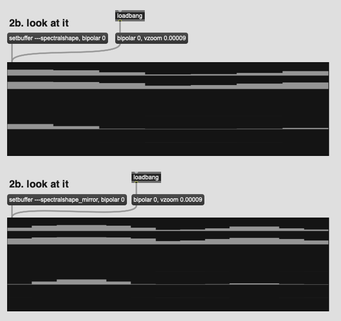
Ok, I’ve realized I did this all wrong…

I’ve been mirroring the frames of anlaysis I have gotten back, and not the audio which is being fed into the analysis, which is what I think actually matters here.

I went back and tried to mirror the analysis frames I get from fluid.bufloudness~ to try applying the loudness weighting for spectral descriptors ideas in a slightly different way. At present I’m taking all the frames I get from fluid.bufloudness~ and then the “middle” frames from fluid.bufspectralshape~, to avoid pulling things down with the zero-padding, which the mirroring I tried to do earlier in this thread was getting at.

In doing that I discovered my stupid oversight here.

In terms of edge-case handling, I think for loudness I would be better off including the material before (and after) the desired analysis window as statistical “context”, and to not pull down the averaging with the zero-padding at the ends.

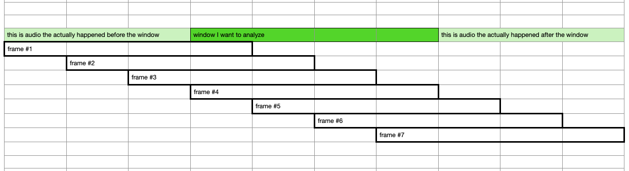
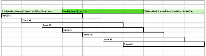
So I’ve made myself a handy chart:

Each cell represents 64 samples and the darker green area in the middle is the window I’m interested in analyzing. The rectangles underneath correspond to the frames that are being analyzed with a hopsize of 64. Using settings of @windowsize 256 @hopsize 64 @numframes 256 gives me 7 frames of analysis, but with zero-padding where the light green is. Given that I’m mainly analyzing percussive sounds with sharp attacks, at present this really flattens my first frame since it’s mainly filled with zeros.

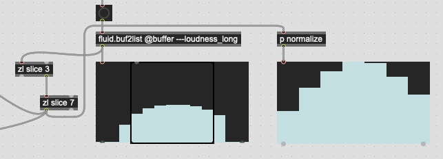
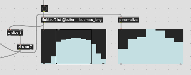
So what I’m now doing (patch below) is accounting for this by anazyling a larger window than I’m interested in, and then discarding the frames that fall outside of these 7. So I have the same total number of frames, but with “audio” in those outer frames, rather than zeros.

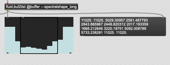
In my case here, this involves analyzing 640 total frames, and starting 192 frames before I’m actually interested in analyzing, and then discarding the first and last 3 frames before taking the stats.

This gets philosophical here, but I think that “what really happened, but outside of the window I’m trying to analyze” is better than “exactly what I’m asking to analyze, but in an artificial vacuum that never happened”.

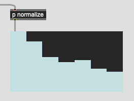
So this works, and gives me what looks to be better results (not as “droopy” for the first frame), and overall higher mean, which is to be expected. The 1st derivative is a bit more dramatic in the difference though.

//////////////////////////////////////////////////////////////////////////////////////////////////////////////////////////

Thankfully, for what I want to do with loudness, I can just use the existing @attributes and a bit of math.

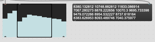
Where this gets trickier is trying to do the equivalent for spectral descriptors, where mirroring would be (IMO) ideal.

Now, I can manually reverse/mirror 192 samples on each side of my desired analysis window, and then follow the same process above, but that would be time consuming. As it was, mirroring 6 frames using fluid.bufcompose~ for the examples earlier in this post took a whopping 0.15ms, so doing the same for 384 samples will likely make things too slow, particularly since it would be 384 separate operations in order to do that.

I’m certain this has been mentioned in the past (though a quick forum search didn’t turn anything up), but being have to reverse material with fluid.bufcompose~ would be a super welcome feature. Both in general, but also in specific cases where you want to mirror audio for analysis purposes. Even better would be an @attribute for the kind of edge frames you want for any given descriptor.

I know @tremblap very much likes the zero-padded analysis windows, but given the flexibility of the tools, it would be great to not have such a “curated black box” when it comes to edge frames and how to analyze them.

On a more serious note, is the a better way to mirror audio for spectral analysis that doesn’t involve manually reading/writing those samples one at a time?

//////////////////////////////////////////////////////////////////////////////////////////////////////////////////////////

edit: I was taking stats of the peak and not loudness channel.

----------begin_max5_patcher----------
9453.3oc68r1aiabsedyuBBiBbauWuNyCNyPteZaRZSAZ11Ec2hfhzBCJIZa
FSQpRRYuNEc+semGjT7wPxgRjRZCjQhWZN7wbd+XN7L+mu5UWsH9S9oWY8Fq
ex5Uu5+7Uu5UxSINwqx+6Wc0ZuOsLzKUdYWsLd8Z+nrqtVMVl+mxjm+0LPw4
13ks7gfn6uMweYl5YiQ2.t1xgXeCCRYNHW4ONjqsPXwHPma.V+q76OZ653sY
g9Yx2HH+rAqjum3E+7qQvhW0cwQYoA+huXHH3FvtmPPTwC.JN2+8q9Jwut9.
gxdgQp.RX1RPE5tGfEZtAq0aCyBRCCV4mT7pJdMrtALBSAXN0HdtTaN0CofV
NfhcYTJE6Z6Bro.6RvN0OiOq4SC0CiymHtCPmHFzt6KM6kPENH+bpKK6kM9p
G1UWcM++KePUwk16nTIdq8y7St0Oxag54M67IlHMP4bJShz.37UZffA6qz.j
M2fk+urxa4m6AFP.E4f5dCh55.P1LByAxfrqsrIhgD+dDfj6U5l6n8XtuPNc
2IF+Tf+yOEjFrHHLH6kZxL2cGWTJW3yVLoeMtxjNLd4i9qVk3ce5xj3vvpS8
kgAKeL6gj3s2+P0yqDjdn8MnF3o1Cr390wqpI5sHNQnEpxYzo4QxDgn2HDMT
LQNtchw6TKQZv8Qdg6zSDwUHHwhq7WGmFuMZ0MbjK+8ekFZlSwI8RtO2R4Uu
8t.thDttmEIaSevO8Fuf6D+4aCii2vO.JN9o3P9g0lr6n4f8fluIz6kvfzrR
V13jf6C3PVl+5MwRL.Zm3wBuzfkYai3XTwP118fmQNtUPzDIqMC0Ihlje1BZ
p5cUJHEve9KiSDO9f3npj363rEwOeeX7hJSZv.jsq0ej3+WEHeEdIuri3lEr
1OMKwmOITOmcPwcwIq8hxzO2ppQ0DaGbgiMO3Gb+CRbHCVh3KnJg9Q2mULGD
XT9Ta4io6lo+6sdEBq0wf00rkexUdYd4LG4bGp4Po2aUFPvstHMNbalOmZKm
CW8NukAQYwoOX8m9t270+8T+jzuNIdEexF+0e3knke86Sh+YNZI8q+iga+13
2480uWphI8q+XbbHmyzB90eabTZlWzuD+52mvexI9q9.G46eyydOkO2knYtv
QoHl42xiAQJRf21UAwJIrxKHm5rkg...WYLrxXRgtcXJIhgaxfaw5V9qNyu.
qUE+zGehx8ivsIhKoj9UaTsbRMeDlxHrSpI8gf6xEIg2n+gUJ17SJo8ddiqS
0O4anY3mD5FpcAEx0+TAeY6YZ+PdN5QOjnUIPKz+Fe+U5u+JhMUlfEiK0opN
H+jpyLRcsQ9Oy0DTZc0KojgVxc964H4WRCRa4RzFKsi2osMnsFeKbktcfPi2
R2cgwbqX5bHFtyPlV0KE9SzPCiPL7ItphbBcgH1Uda1T4z0js3HxeNV9fbtt
7TAQpSUJidUhuveE08yJOqWBGOkwQRaSTn6OQsuZ2igyXlDsMnziOIIsTYHm
3IHSoa7VlaWhSiKFth0NnzMHGULoJOTEgltiMi6uhxunJJ74X6M9bYlMI9ob
UKdMrevUP6emGO9paq4tJ5FsieW9LT6fkrZ+9j.gst7K49jfUwQhIQMJg3zE
uNtvhz1MjTEXjWQj2FM2LmyPnxW+fBkmaSW3kHcrTY8CULXlvnPsgJuuP+6x
xGdSPTTCrXV7ltGLQXOs6gWDyGbceOa4Ho2tMRM5sbdBtU.umpisy3pHykvq
+3+jWTvZtIiBM+bqMEC1xoWX8QdRyHq373K8eNXkR8OnJy.+xC1TvDcUIUdU
v8byR0OWlmxyycmoLx3JmZaQLA2JzpFla3a2EvkN3NOl9P7yo4WXAiVUDfeG
9SrScYC6n0SvfeZp28ULbWQ0HFBIvapNjFshPhTbjPkp.U+QUEgcqLriDDT6
FqnOjbU8GXivwZXJ458DenlOC.ytNxzAPbugV4GBj6KtR4DFzKB.nGBQcBgU
wXEw1WkUQ9fhV4+oJ5YmDzQMqp04NtKbavpa7VuIkGzo+msd6CbUAa323cI9
+agbHv5sbqawIVulP3Gxkq49luY6FK7t+ZU7yQVXG9YR4tXjONBAH6Ng7RTm
hiQjuLk2RVPtMXq2x0+9.WC+CwgqrfP9ee2c6NQMllvfH+k7fGkyeb+jXrsJ
OHbKOUowTj60V1.I821sWhLpOt7JQE0E+NratgIj.WOSQ0ovbqlqrR4jfPeK
I2kUVrUgdPNc0qtOSswwngTcnviTvM1tU9wFyQ7Ho2VX79HHAQmbb2ydAYVY
O3akyqFeWI5x5YNxL948FqwjdLfQPMXM.4.vZfSNVSJyViiyiiE4l1E3Odbo
00LOJrlijWCwQdvpxyNTAVyc+wZNmbjlL9EN5Zy1grawsmeCWvBwiZA6v+Mh
HTlIskIWw.zdY1BeTv.8XIZiUdJSG.5wxnHrgMLayP7S5La9s3zM9AzbBuKb
t5nhNCqqqP6Zb65Bwqiv75NTugC2qqP9pE1mAg90L7OTdj2x+wNmVY2fYUeL
fFDGnIwBNX7fFFSXOwEZVrgCDe3fwHNXbhCDq3vwKNXLiFD2nIwNNl3G6IFx
Aiir+XI6Odx9ior23J6J1R8wW1QLlFEmogwZpOdylJZZpNu03CZXqtt8+PTJ
WSSJ2UJtm.BVZ9TL6yVYdOJOI2+JN8tvkAtSBhS8Dm6m6dJ2YUumhCVIbffa
IvJHMcqe5MMeUcEUPmK8BzovaAw5jJMeZyZHh1qwy9h6qGin0LjV2X5gREZY
bsgA1D+MhXAZYlsSSs4qCKRrf41TnsC0ARsATjHwc5L01u4VCL41DoxbO2wp
u1BZNpjwtwgvv.lMOxTGD.C43PW4p+MAXxfnrdQlNfdQlnSOxzakxnlEOx5m
RM.uhI6jhcXFxRhFjk7ZCPlvSNxrUVtFRPlGe.gAc4xxLjCARDBx5S003T8g
6WHswfcj5qNR+kF7Wc2nDZ9GvXlDkHtt9QtowaSVVvCTPisfsvKbi8YAQd6V
EtRoKwposWD98dFBpVqCCLCEJSO5yvhWpQyP7fSvJCVMVjqD9Jt5VkOy25kk
kDrXalhuPWfX6k+Zp0NsgiUc4R2W0F.l63m4B7wIqDKub+gP6nRuOOPZb0eD
odh5dnQP2nneZppvEaT5wuDGcmwQSTKSMFoV9Bnx0Uvk3nuDG8k3n+UdbzK2
ljvGuHR4MwoABTk0BeQnwOmDjk4GwCY9PiNFCgRcL7+wAy0zfrY.FOZEQplU
peNrXkom7n5FBSqOc7cguXHQLbpZuVeR3GG9w9rG+7sI9bIGKOqrmisR4LWQ
qr9mWsJdKWz2Zw16tyO4edkH4MJmRrhi7KtLwhnIwtYOy0DXkFa87CbtV4Bq
8KB9XBDkygmdsHUPI9VAoVdgO68B+erdxKLXk0xG1F8XkmUb9Cvu+TCYOBle
IcjHWtAJ3W0oFRQv9r0qe8qkqOWpbk+ad48aHuCro56xAykGvUzj.nNhDKMY
QrqJ.OQkg6IptxdhaGBP5fqN7x4bjXwA0URvz.8RNB8RN3aH7eDXdGaBf.oJ
F5oIqSChwsgm6r++uVvalDlcwmrhKwACXt.D.5fPBtbmafPHv0FRnt.H.ilx
j9UuzS0ywiODN9yfzBtJcirhx+7zPjHjaPtPpMDgI37zfoUFAanLhsIYl85J
Zox+6gxwHTuN3ufzUsI9Q+JlUlF5m3C3iS+PDWFkS7HpBBgw+gSOcQHBhP4j
OWjgjudrb6RNDB.9zS.9+9rksMmOZhzuwbkhNUQ8b+jPHDzwACwNbsdhuOUi
kbFT8llzI0aJk9RT8lz4zOaAlRJkxxOjGXhn5XpopiaKZpL9X.0ww4Kbpybn
BS4T7ro0hPO20ZIealfnpDJlwqT0Tv1h6ODbPOqoUOoNvnk25nu7fHlcSs5M
iWSl4mIYoBI68ZEtuI+57ZMEcwiX8vDteHV.xi6ZJ5LlYndvYcvpMwb2ayQh
4ksKz4Fa9OPaFylvnNPQwNyGqo2bsutVufxOic34KtQnFVyxGWN0QmuScgXp
wjU.4FYiIA5Pv.DCaK5PI7.pZRVaeccia.GUbiHEEFia5.QtLNTs3g4esw69
k7Ko8nBOBqWiSIy.viacB204mB6BbrA7SJOCf69J2nAffPLFgccyOgXcrPDk
unTnrf9q6mJA0JXi1W24BKznP4RMCGMT9IRWoLuSiyPBb.oJhKAvYFbE0NG0
Uf.H.nKhiUbXtXnCRgkbrI1LaWhiMz0wH1PQfs1MSbGEHY1Hj7uMGGWQ3tsR
9flq6bgobbj.ohsiGI3jwVBFQUc0EFbxPJF6Spb8rGvozcAhJhA4CxBa3124
GsstOwEklQ+XtE2eWPXXIf9pNuRdvx4wVkiVttwv0PVHWaHzQfPvPLCQkGwO
fPzPUxuWXwMyQfbATwsXS4gsPjG4HLFbskl3Rxuczt2Mmrndi.WGkJTr3TPs
rnu5Jun6yKHDFnYTybVvj3MwIkUPyMX2V2+1r36S7VEjGDSMw+5z650DjpK3
vuK8kwfPClnox07Y1m.SIywOrco29vPTMUGbwi+5Fd3VevKJ05C9qCVDGt5p
9ESrYDHVRxPbACW0QDnThQmBBQJXjOfaChDkzUYSgAgcQPp51K3GPLGardxH
mSttkUtUSlTJkOI3wXHOxF4xjyHBUy8OdIgRp9.BCijgrt3fSoPfCCPbbTG0
Ihno3.kq0RdOxOgNl5H0S7jHMz.sm5Gp50M0PYLgJV4rFRYHkbuC..s0S68V
tzOJq1S.K3ZjXZ6BDfP+icGrg7Yw5lOBlCGeoP7buEbTGweZR+FZqV+HIX+9
eun0KwerfIP7VkKyA7QkHzlqjZrY.IirfOFOVI51wKMjHrRFQ2Q5t8kg9dIU
dBP0KykK8STR.bAHFtq28uNE+G8sejk+qlz5eRl1ZSjtGRo1IQx7QU2e8GEU
K79Ha1j0s1uNQvzZuOQaTlxlBNSjdfFnBtVHSXPT74ktPvxk7NsHRMKHxn4L
3dXw8DF4V0flvwHaB7TCdsaPQGEdkoVucEMuE5VZejAZdYNhXVtV6Qce6+pH
JF8ZMNLtKcqz0dH8H4kpDgYUGYNIRNpUl9aB25+Z39.c578Ex3dpIMJVBnth
SAOC.zj3milLHcG7QJ0EhOSfzu8EuoCPAHdTrJSYLLFozEgfPH9zCneehu+D
BoRpo7iUSE+mvC1SOP9NtksnLuICLcrATpJvVJ.Rk9qvntPWxoGV+G9htH69
Aps8mm3B.NF4yFh.YJqjPGYzdhbtdZ8oOZ65E9Ieeb3pIixyJihlvcOkHgXX
UK6mD.MQE7h.ROXarTawlUQtJJVdt23DRWrQw8edhf1ge1ONgFo1fAAR.yEa
SAt4YmjAIFmfqySrTl2lIHsT+fWVr0On5+6y.bb46Kuquub+U2Wq.769KKWe
uYCYvWVducaS027hlO3j5kLO4T2H6J6uQCfrvtp9loppXp2AHUsJ6C46vu82
ERczD8nzHd6AMs7ANczPNJLCWuWEHx1OgLy8p.tZ3SMuzJ+PuW9rEhPE+uY3
JDsMCkKb1wUNmZFpTuGLiaB4.p2NfUsOTTqtp4rhubOJ3ql4UrG9FR2EY8TB
3HlQcRygqn596U165C+sJl2c3Pc0PRELoAEuamkMRidsSujxwNMbLeZzpDTm
9JWYRAMI6gQvlFZwzW+bZJRoSD3BOFPay56U9Up55111K1tigzi7.yCxC3Zr
bPqZ18bZx0pZP0SHvPh.cCrcH.DkSLkswdmNF5nxFqA+1EvxlQEikOcClGjY
cdPMbdPZoed14KMcpgFPiiCgfYDjiqKj5JMc..bKGLLC3xeKpJKfqCBJ9lpA
PGUcxbrUvBHGfXng0z+zNiGkKFv9TajqkVzCSZoAW9og1ze21WXG6vW01Pb5
v4JCJFUMY.pBpoi0usZdV5tvS22hN8.J3zCnXS6dIZ6e4Y6YoYqlWnq+pgyJ
V6LhoiatihHseB43Jbz8tnQmjBF8PJVzQwwpqRC1+04+.pLr8unPmEt1pIc8
.K.zCq3OOrB+bVD5dmWV1XD5J5Ki+TC6DMVINvrOw0UYpiRmQ6pQcuqD08qh
hNfJPcuq9zeUnOYT25LqPo+JJ8PplzYQp4G+3ebOEW9SurJI9d+nOJ4N9WMy
+mpk3Uk0P3VjpnJPh1Tkh0fSsT4+oa4NnvcJkoPgvl7xYENV0uDDjhyKEIHy
NOBB9Q.2yX4fQ7oCbt4MX2hANCKFP.LpJERTBVUIFPNmBxPql1THOPLUQ0gn
14KMMjqF3XHFIyFd4178XEk9d+H+m7LQHpWyG0wG4VlzczrXsxA6xJp64b6j
hSQNPaNcD0Eb7u1CRboInl6qe6iNHAMSjkbGVTZPZ+wPV3a1lkwgLCkHZ65h
SI4AjezQap+c0ZwReAMw+dufnOuGybNuWoo01Gc7l9oOK1A5ME.Zw4222sxQ
Xdi9hah+mUkU19xq2XF2ssgdsinOD7wX+Rq+.mC5.+A+U6udjtvW5fVZOINd
9.u24kkD7okYIgSDTdTlz9Y9Ie17DDON0jeIvU9WhW4mtWVIFgiOC30x4KxY
uUIBNQLz+EYQha5DVm111NtbDm9uOXY13v4ms7NuWrg2j8EomieXY7F+8y0w
cqZka42MyvtDbVPv9n2h8CjOPmSFTO5QA34Q8u3fBRqa++55Kq5nqb7iw2KB
+dVBIZ.hbwWBn3trkKHNmIIeIcOFf9ee8HVH7yffQ9Qum7uKNY8mmcp03i3P
9c+OqHgUdIO95HwGcxqko9yTjf97DZuq2CTtXzkKKsiDnzmAv8XIUlnTmCGP
tY1xl2rk1b8YySipwAWYwYky6my+bf.fJeYYywiGsuKL6hPetUJU8b7MwwOZ
Rlx2spZsNn+UNs2UfALiYx17W6Wr79MiIjL6r1AQOdXZRojqq86NW6jxafi8
.NkN6fohs6kAVrFCumlq3xHzQ2lKe2xpJea3pGMCKXy3.0SfMgSRgFYHgWWU
CX1cpMYg8bqyp3n9VT04qiogB2wFWHRMyWHv0NufBkeuK4GwbLLPQi6vHyB7
2pQ5zOrOAKib+saq8sUaMaHmFe5aiICBF1Fslsodq1k07PamzHCFSKw5.ZGV
GIWjlxZrtsj534HZ1hqFahuGnsVMKbx5aeUib0WGQKqZNAhlslpQCEmViE5a
6TiFHLtUSMi.QqVJ03gBCZiTyH.nocQMZPv3VD0LBG+M+UGDLvJCV.VFSMH2
x6wBFZ2NqFN4GCzBqNf1W07CnneMCnZ6GWimszzlmzr.Da1lrI7vc7iU9MIH
10gcTqgkPM2vkkMFXCTN+hH.pqT.E4PnniRs5l3uzO3Iyq.Bc7fk4aYGrCNZ
0ru1lk1H7VaDMHs8t4nMK.dpezpzuDsJqu6sMBR1H5XameJbp0U1FUl+01I1
lo4XZl+caCCy1+ELV7A.yjXYZYLihTswbF9CUwgPfpkoihYX02QJkqRgdbHP
Jf+z.6HGlixQSbonIF4h0roNcFlirLQe16KwuWxmEYg8k8Tv76BRxdw5Ober
IKEGz0EnhefyPamWfST..Ca+ke0o6Fl+MC2Qp1ABFTYdev47kb8h4K7Z+0tH
lNMDi7mQwCXnF9XN1uyF8ntl73.M3wlM2QUxkj+VwqHemU56Wp4PO8Gsc8Fs
Eau6N+D41XcX71UQ9oo2ll4kkdaXbz8VuUrm5lZAK1zi00kvboTgMZGUGBCg
cZ1Q4z2KG6pyD1rQNpcyWVSO2aZvG2EtMX0MbrhDI7YNBP1FNpgexwLhKna7
VlWRlnSFZArdKexJNjiGyG3tDNM1BKGQdbpEy5sKBiW9nXKKFIGf66QvS76o
XNpjP2pR0Hta5AykpZUa1pt9mr8sY61I8.2E8nnuZVRWzSSPyMMYiUheJWvL
8iweWvxrdXEsYpVmoKVxQ5N.mHrKHeUfTSjWxK5AYfdPt5DyOooFg6BB8EJG
y0HTzq7txaylJmtlJbN54mU5Bctt7TAQpSU1r83wF8TPw8yJOqWxRgwhkYaS
T5S9Dc2dW9Uqi47WQaCpzgcJ0QppsKgdnzM4F9tpRdpuZGBmHQwPEqF0V0kW
cpV3Cb+FDr09qp1G+tJdieTPzFQk2FkU1.aJGN2n1scr6zWa7BSyZGbWqlIo
xWG1U2mDrJNRLIpQIDmth0bofi326.F4UD4sQyMqrHzwfoxlbyBuDAgZQ9hM
TpdONNr9Pk2Wn+cY4CuIHJpAVLKdS2ClHb.u6gWDyGbceOa4Ho2tMRM5sbdh
raEV+pecdgg4xs0e7exKJXsWleVfhDf.kC5G4wAzG3FHiCCqAupQdRyHq373
K8eNXU1CpkhoB8dDVZ2YJsVmJpwo1tHWF91L+0aB4PQ8KPT4ioYoOD+bZCi1
UQ.c0+iLqAc1dmwYmFwDe9jhaU52fs9MPqeC2MZkt5d6lmDUG7LmsFiOzF+Z
mcxSh6otiu9ywAQFgMPNJak1z4CavN4MT430K39NXIcnfqr8I+z27FqHq2x8
c8964ldrfC0QpYLI9gHQS7HCNzV1cMuIZgwvmZLVl0BKfQLPPfRpxdpZh4AQ
c2btInScamV5+Y0u4mdYWPxxAgZRKl1tObi.mbcNSy.nH6t61zjiCJhauza4
ibCTs+OyTIovZXjIrTrg6z6WuWGzI9kdpYAyrBsVXlroKxbk6Cptp2cW.6S9
lKvuDZwc1OwhYFpgVFU3LpH219j6HPZtMNqeK+pr9FY1N9s+O5iZ++42cyFe
+G+sv+4+7Z.++sf1+temYnSUROvHmYyMBzoeKGXWr2C3hosDMv+Cxgo2uRX3
UT+2MJB1M619uis3udQ8PiJxgH2iet.2spPV54BVyCvu7RN56NKBb3MRKRq8
8hdiUZ1JdnT7+8Q+mE7+uw5wsIYw73YdiUX7yuwZcvp2X8.O3w2Xl4JkOglY
tBZH0t68HfNovrIDcVrECnCeJLCX87C9QVqhi7G.EAgUcRL2sYvPeKBptlV9
uf8hPA5wSX3QQYgI6gDJtDavzrGRzImAkL5MOBi2wH1WzSqcezdvOXyQPcPy
o83Y1ghAlk8LCpoMfaBZF6H6DS6F+H3bNKLs8zSlysODhoaeHxoKbtlEnVsu
b8yBQrdVn95y4LaoJTDUoChU9Wy4T2Hlo4byNv1z8bAI8t+FEuCU0n3k1hHz
c+0bM2McSH.NmJEroFxBBQynffbVfLcVflyYA1zYAdNmE1lNKrmyYAwzYwrJ
iPMcVPmqYAYLpoAy4rvD8EEJVlmYgsoyh4bykw3sLpho67LKLceJgNmTDHZL
tx.5X2L4WEU9iLC.OE3+7vENAAmmcPlJONvNKcBflph.d9THHX.9XTHHT1kB
A4RgfboPPtTHHWJDjKEBxkBA4RgfboPPtTHHWJDjKEBxkBA4KyBA4fqADj6k
Z.4RMfboFPtTCHWpAj4oFP5096k5.4RcfboNPtTGHWpCjK0Axk5.4RcfboNP
tTGHWpCjK0Axk5.wn5.IutINn5.gBl65.oylViQ8qFFjcCyE5xntxebD8Ssh
tWCvc95dMH2SAhoVe7AagLnS9..23.bIDahC.inTQKBCAoyHlgdBvLEHEVu3
D8bK5vPPGvLhgbNC57Qc1zi5oeGMQM0HR8dZDbd6oQHxjgs23E4G1C+kiZQo
HX5MLt9VGjhMykJ1NDPx0sBVMcgCq+EUrp47YVxJU4mgpcFi1km0WRahpEq5
6UWqyuUqB75Z+Z2anY20mLcby+RnUZX.m8k0qrM4FTSYahCoMkfP1WQ6N4wf
56kYnY.Gf6AGPYtZvA53FmCb.dtwAuVr3uWMXyRCRTd5P22BEsZoHTCBgSFD
VuNv1AhU5nb+FXsB.qO.1UBvPHdegXsfq6bSOKsRUX.plgp3nTeg0n678DE6
ZpFGgdNHZU7yhh6TrrUVu8g3Mx+fZWsa7QsAUMcsmsfODlcTZAevoyiaYCvr
1F67Uk0c6v.rV8FnbqXPmavb0LhtXssKvlBJSiyUbpFedymHpm1qYEVjFPSi
fZWT0lvQq8gtSLoyEx8vwn01Ip5A2YSTqdZ4uGq.Y2cMSxQAPqKw9j2tvXKE
ZQgAoY+D7e0sXs7J3hdR20aI9Z.VTUw+HHbR0qgcOFRXrd7+k8km7kM37P.S
g6lO4Ka3Yk70dHbMLxSIVAclVwJa7zIVMIdGQlSmivmuNGYpeQxg1e+hH0cK
ZlihGOL2k71pWLCJ7ey7LmSEZmeYP07K2QtkwUVixVTZSeSXjIuIxD7lPDCd
S10Ru+UkYZ.N+uZJS+qFbX3WrAuZzTfecM3EUvWcPunFHpNvlSwax1Djm8j7
lfl7lvSg.mIzI5rvJZDGBdND.wlH.hcmBzqQZNgSwaxjWzTvwXhFZn6rn2zz
2Lbp4UM5MCczCznC5U23odLw2l+pmbDtYu5YBiaahnDXNzIZzqFYOKD6ZkGW
WXb6IPABzHh6rn3GZHe0rPaMwldaaNJm2az0DDuiFcKgFcJg1cIgt6PBM6NB
xZ.Q8kh2HfgcMXfsqBh+f7y7+124GsUECRi8oo+SwBk0Zm1tn5QJ2gsUiV1P
FpuIWayIaxMGIHlgTa20hclbR0Jxpw1wckM747chI9QhsTabsLB0bq31zMTa
8al1cuQZ2wlncQEtbcNijtcro56VSUY7JIF+v1kd8Q.ZrAY8W23GY8AwJW+A
+0AKDaUikbk02H3YDnZ6HG4hcbUGQf.pa80PsyMFKD1EAUaXbkzCjbius9Cn
wRo5BrgL09HnKwNeSfzF4xTepHzJ22vbVM2612ucP8V616ELU61tMcZCXMYu
LbiBax3tJSvotMcLFhSHcTa1jLjRtvA.D6IwUoM51RxK2J6J24hw4aucUuSc
aHdLGNbqPb.nii5H9SAgprg3cvBDuyKKaHABMa1cctQ2cvSn2+6ytUdafQHm
pZhK5EMcy2c3DhCE6elfpas8CIZ1YAQzRVrXqzs8QUuskg9dUK4Bn5g6xEeI
JVdtjBC27c8kk7qw21DK.2d6ntOwygzxLIbz+3G+iifU9O8xpj368i9njp9u
pl6zVaIiHgYd0lfKBRnJEMBrMp1VxXc9.nv0.k4AgPf7RYENIzM2Mjh4hOx2
Eyl55leDv8LgO0LMsmbuXzyl5zOaJAvn1p8aSBVssoC4TbjAVQroPHP4SmKh
Zmu6ACcXNSIKtbkHBVNB17u2Ox+IugXv6T0acXLWattilTM7NXW0NNJ+fbaJ
hSQ1Cc0Z7hGNtWydyJ2Djx86r8Q6k.Pe74t8ylOHcbJ4U+lJqRrdN11lncJQ
wf7il7o02U1M5NilTeuWPzmMbVw4AJMqz9noepk9b.WyQeStVbZvbw7c+ZVl
SnypI0etZIlXFuUiYidchcp6TenTlpqVqsrio9geve03jC0gCztQm25hmxoM
OdtjfOsLKI7.l8S5DRT9Ket+jdMN0GmKbH+k3U9oFqUzPCs8Xw7zCviREBXl
Yr9KaWun+IiNMPsMZNCSs2GrLaXb0Imd9dQW1M6ryaiOrLdiu4tarKq0tXwO
C6F+QEI+QuElCJGfwwA0uLo.EORpEi1AZ89SnIPf4UwwGiuWDJyj4NaODELO
tcFTcG1XnLlL67kUYJAo+95AVXoinil+n2S92Emr9ySNFd7dTV1ORNXfakWx
iuNRz4resLUE8Ab5ykgcoXIqbAdJWpGG4DtclJFY5TOfzuAGfmcxy7vjm5s5
YdPiZkAWIfIgS4my+n8Af7x.eJdTnwrXHKB84ZlUqa42DG+3PYYaWVvacP2q
ZQuYbELgYCyrWyWD7jM8smLYrbAQONdMRTx009s1bkVdwbr.vozvLlB3pe5I
orFb8Mytpg53ZyItaIMjuEb0ilfDyZNHcD0kdTV3aCHh5VUsguKsIFomaaRD
SdTES1OJJsmSsyRgBWIF1E5l4FA3ZmWbIttXGV9QLGCBPfV5rAoT8YA+4zAW
q89DsbGgQOLcfKCSCRhzEut4EcpGQDKWnZZA3J87TShxCgIH251wDZ9lb5Ps
OApoiVbvdX5TtX6sOpGUiLGQUocs1iNhlzOj5TqtzgYTwpcKVSS5VkZ5ax8u
U8sl8Mga8eMbTqvgnpDY40PvNkQtStJn7IXR7yQidFdbTRplge6KdieBBPtD
0p3yXXLRI6ffbOfl9I32m36uGyPI1qLUbPpvutoex8NtlsnLuQO8brATpJIg
T.exIQkTWnKY5mi+M+Uid9wJcTDVFuCH2hwTO+9G9ggwO2+TrcAUQbA.mds4
hHphTg4.cjd+xuGhMY1..zWh.fb4K993v8fEoL6EDteMDU8.U0j1jLA2rMYS
3947.qr9GsgDt7uTIkPMP+kXFFXCTNFgH.pqTH.4PnnIsVkR7W5K1oqFqdix
XR2ASfIuVASTgnHXKL1hO0VzhGxMDvxqAbN2pKtWr8wgKJ0OZU54lEjcH49k
8ZTduLHfoVmIaJvMuT6YPxfADebP0YdaFQVB+AurXqePDE5US16OMy+tsggY
iaAVDezJLI1gV5qtHU.kknXGEjpCg.UoQmhYX02NAkKRRmVjpBnNNvDxg4nb
NAWx9iQtXWmyk36y7SOu9dAdVjMmWFAi+2Ejj8h0e393gRKNz0En7OjyTYmu
n2T..CqWc0cZFzrugkNR8FPv.IiwEmy2v0iju.FcWuHX59gXUe5bcr699U+2
u5+2aVhky
-----------end_max5_patcher-----------

[tremblap]

@rodrigo.constanzo

This gets philosophical here, but I think that “what really happened, but outside of the window I’m trying to analyze” is better than “exactly what I’m asking to analyze, but in an artificial vacuum that never happened”.

You are right it gets philosophical, and that it is only what you think is better. If someone like me think the other is better, the current implementation allows you do to both. the other way round wouldn’t. Ergo, a superior interface design! This is as if we thought about these 2 options…

But your drawing in excel might help people understand what is happening. Which is a good contribution, so thanks for that!

[rodrigo.constanzo]

@tremblap

You are right it gets philosophical, and that it is only what you think is better. If someone like me think the other is better, the current implementation allows you do to both. the other way round wouldn’t. Ergo, a superior interface design!

Well, options to choose would let you do whatever you want! At present it’s not possible (without some tedious workarounds) to do any kind of mirroring, would be the other most common thing to do with the edge frames.

[rodrigo.constanzo]

A question.

So I’m trying to do the same thing as above, but with spectral descriptors (centroid in this case), but I’m getting unexpected (somewhat) behavior.

It looks like if you analyze digital silence, you get Nyquist/2 as the default value. I guess it has to return something, and this is, I suppose, no more incorrect than any other value that is returned.

But I noticed that if I did what I’m doing above with loudness (analyzing 640samples, when I only want 256), the outer frames, if there is silence in the buffer, which there is in my test context, are filled with 11k:

That’s not always the case, as it seems to depend on what else is going on, and what else may be in that bit of buffer etc…, but contrary to my expectations, this approach of taking a larger analysis window is biasing my queries upwards towards Nyquist/2.

For example, here is fairly bright sample hit, with a mean around 9k (which sounds about right):

I have no idea what’s going on in the frames before the attack, though the ones at the end seem in line with a decrease in centroid over time.

My question is, what happens with the zero padded equivalent of this? I have no way of seeing the “zeros” that are put into that part of the analysis since it happens behind the scene, but if I do this:

I don’t seem to get results that are in line with those light green frames being filled with 11k. So is the “zero-padding”, with regards to spectral desriptors, doing something other than filling them with Nyquist/2? Are those light green frames filled with a centroid value of “zero”? That would be more in line with what (I think) I’m seeing, with the mean getting pulled down by zero padding.

What is in those first few hops when zero-padding an analysis with spectral frames? Nyquist/2 or zeroes?

@rodrigo.constanzo

On a more serious note, is the a better way to mirror audio for spectral analysis that doesn’t involve manually reading/writing those samples one at a time?

Also, with this it occurred to me that I can also have a double-buffered “reverse” audio stream going at all times (driven by the same count~) , so when I detect an onset, I can fluid.bufcompose~ the frames I want (dark green), and then do two copies from the reversed buffer into the the mirrored frames (light green). A bit of a faff that, but I guess it’s possible with native objects.

[weefuzzy]

@rodrigo.constanzo

What is in those first few hops when zero-padding an analysis with spectral frames? Nyquist/2 or zeroes?

Zeros, because any padding happens in the time domain, before the signal gets anywhere near the algorithm (which doesn’t know about padding). You can probably see what the results are internally using framelib (padding vs mirroring)

[rodrigo.constanzo]

I thought I understood this, but when thinking back about it today, does that mean those edge frames are super pulled up towards Nyquist/2, in the same way that I’m experience in trying to do a larger analysis window with potentially some extra silence at the edges?

Or does the moment there’s a tiny amount of audio in an analysis frame (frame #1 in my spreadsheet/diagram), does that break the “default value”-ness of Nyquist/2?

I’m just confused as what the difference between me “zero-padding” by having silence or near-silence, vs the algorithm zero-padding, if it’s all happening in the time domain.

[weefuzzy]

@rodrigo.constanzo

I thought I understood this, but when thinking back about it today, does that mean those edge frames are super pulled up towards Nyquist/2, in the same way that I’m experience in trying to do a larger analysis window with potentially some extra silence at the edges?

It’s possible because, as Alex says above, the zeros can introduce a discontinuity that can, in turn, spread a bunch of energy over the DFT spectrum.

@rodrigo.constanzo

I’m just confused as what the difference between me “zero-padding” by having silence or near-silence, vs the algorithm zero-padding, if it’s all happening in the time domain.

None, I would think. But I thought you were doing your own mirroring / folding instead? I’d suggest that FrameLib is the tool for this kind of forensically orientated work (i.e. you want strict timing, and you really care about the initial results from a small population of frames).

[rodrigo.constanzo]

@weefuzzy

It’s possible because, as Alex says above, the zeros can introduce a discontinuity that can, in turn, spread a bunch of energy over the DFT spectrum.

(aah, it’s nice to be able to properly quote formatted text again)

Gotcha, and that makes sense.

Out of tangential curiosity, is the Nyquist/2 thing the norm when working with spectral descriptors and silence? It makes sense in that, it’s probably mathematically (?) correct, since all the frequencies are at equal loudness (none).

@weefuzzy

None, I would think… I’d suggest that FrameLib is the tool for this kind of forensically orientated work (i.e. you want strict timing, and you really care about the initial results from a small population of frames).

I should poke at this and see. It’s just hard because I can’t really see/access the actual zero-padding that fluid.spectralshape~ is doing, vs what I can feed it with a larger analysis window. So it could very well be the same results, just hard to see. In running patch above on general demosound sounds, the larger window gives me visible/readable Nyquist/2 at the edges, since I can see them before throwing them away.

I’m still quite green at framelib, so it would take me longer to figure out how to start building something like that, than actually building something like that.

@weefuzzy

But I thought you were doing your own mirroring / folding instead?

At the moment I’ve not yet done that. The tests I did a while back (above) were conceptually wrong, as I was mirroring the results I got from the analysis, rather than the audio I fed into the analysis. It still did something since there was a stats step that comes next anyways, but it would be (I imagine) very different for actual mirroring of audio.

I think what would take me the least amount of faffing will be to hand craft a couple audio examples and just analyze those static things, rather than working out the parallel/reverse JIT audio analysis which has to concatenate the perfect bits of audio for this all to work.

[a.harker]

I’d put a strong vote in for switchable edge behaviours as part of the objects, because although I agree that the current interface allows you to get to lots of options, the process of how you get to them in a musical context is important. I am wary of comparisons between things I’ve made and parts of flucoma (because taking things is not a competition), so what I’m interested in here is the logic, there is a very clear reason (from my perspective as a creator) that I decided to build a bunch of edge conditions into FrameLib objects (even though one could prepare the frame using other objects and post-process) and that is because it is long and tedious work, which I frequently get wrong - and involves lots of diagram type work (as Rod has done here). I absolutely don’t want to deal with that in a musical context when I’m using it, so I hive it off into a technical area of work. There are also not so many options that make sense, so to me it doesn’t make sense to have users replicate that work with the possibility of mistakes, as compared to building It in.

[rodrigo.constanzo]

I obviously agree here, but I think this is something that can get easily overlooked by someone casually, or even somewhat-deeply using the objects.

I mean, I only really know about the implications of what frames are getting analyzed before/after the chosen frame because of in-person conversations, which most users won’t have had the luxury to have.

Same goes for the zero padding and other “overall edge cases” that happen as part of the system at large.

All of that to say, offering options with friction leads towards no options being offered at all (and default choices being made more often).

As an aside, it would be handy to have something like the bit of code I posted above in a helpfile somewhere to show how to create other edge cases by just choosing larger analysis windows and dropping outer frames.

[rodrigo.constanzo]

Revisiting this analysis frame thing today. I’m trying to build a kind of slow-mo envelope generator by using the loudness (and eventually other spectral descriptors) on a frame-by-frame basis so that a single attack can yield a variety of envelope contours, and when unpacking the loudness frames I can never get an envelope shape that seems correct.

So at the moment I’m doing this:

And throwing out the first three and last three frames, so taking frames #4 through #10.

My thinking is that there will be real audio in frame #4, as opposed to being zero-padded.

That ends up giving me attacks that look like this:

And this:

(that’s normalization in dB and then converted to linear amplitude in p normalize)

So with this, the loudest frame I get is frame #7, or frame #4 if I count from the trimmed frames, which corresponds with the analysis frame that is full centered in the analysis window itself.

This, however, is not the loudest frame in the overall window as these are percussive attacks with super fast onsets.

It makes, computational, sense why this is the case as the loudest part of the analysis window is generally preceded by the silence (digital or otherwise) prior to the detected onset. But this isn’t really intuitive as, perceptually I would expect something more along the lines of this:

I’m thinking that mirroring here might give a more (perceptual/intuitive) set of values since it would, presumably, have the highest amount of energy centered around that hop of the analysis window. Or rather, folding, to use @a.harker’s lingo from above.

I think that would require dropping another analysis frame too, so only taking from frame #5, which would be the first frame that would be centered at the start of the analysis window.

///////////////////////////////////////////////////////////////////////////////////////////////////////////////////

Am I thinking about this correctly?
What’s normally done for short/loud analyses?

Up to this point, particularly with summary stats, I’ve been taking the mean of the whole thing here, which, if consistent, should correspond to a comparable descriptor across the board, but if I’m interested in the specific envelope and contour of that short window of time, I feel like there’s probably a better way to approach this than I am presently doing.

[a.harker]

You are unlikely to see a shape like the one you are expecting. The system of analysis is symmetric in relation to a ideal impulse, as the important thing is that the analysis is in chunks and thus the impulse either falls under a given window (chunk) or not. It is likely to fall late in the first window under which it falls, and thus be significantly reduced by the windowing. The highest output is where it falls centrally in the window. Overlapping will adjust the “pre-ring” (more overlap gives more frames of “pre-ring” and vice versa).

Also, although the window reduces the level at the edges, at the 25/75 points the level reduction is likely smaller than the effect of the sudden loud transient - hence the relatively flat output overall the peak in dB.

The shape you draw is what you would get from a time domain envelope follower that has been biased to respond faster to attacks (and therefore is non-symmetric). I suppose you using a super short FFT might get you closer to that (but if that then why not use the time domain)?