Removing outliers while creating classifiers

Ok, looks like there’s details of the workflow here that aren’t clear to me, and that I’d missed that the motivation for using an MLP was with respect to the furthest sensor (although whether or not an MLP could deal with that depends on how the data is junk), rather than as a way of avoiding having to find a closed-form expression for mapping coordinates to arrival times and, possibly, dealing with extra nonlinearities in the physical system.

In my mind, the data flow was just [calculate relative onset times] → [mlp], but something more complex is happening? I’m not sure what the lag map is, for instance.

If the most distant sensor is problematic, then it’s probably worth stepping back from MLPs and looking at that: is it more noisy measurements (so, stochastic in character) and / or added nonlinear effects? Having some idea of what’s causing the dog-shittiness should help figure out what to do about it.

Meanwhile, with respect to the MLPs

Really 10 layers? I used a single layer of 10 neurons, i.e. [fluid.mlpregressor~ @hiddenlayers 10]. But it may be academic if we’ve established that we’re not trying even vaguely equivalent inputs / outputs. In any case, you usually want more observations than neurons (so 9 training points isn’t going to be that reliable), but if it converges significantly worse with more training data then that points to something either funky with the data, or a network topology that isn’t up to the job.

Standardizing will make the job of the optimizer easier, but shouldn’t necessarily make the difference between being able to converge or not.

Can you just send me your raw(est) training data and patches offline? I don’t think I’m going to get a grasp on exactly what’s going on otherwise.

1 Like

Ah gotcha, yeah should have been clearer.

The whole process is such (for the 4 sensor array, but similar for the narrower 3 sensor array):

  1. independent onset detection for each channel
  2. lockout/timing section to determine which onset arrives first and block errand/double hits
  3. cross correlating each adjacent pair of sensors
  4. send that to “the lag maps”*
  5. (find centroid of overlapping area)

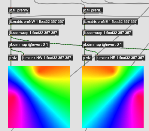
The lap map approach is something @timlod tested and I then implemented in Max (with a bit of dataset transformation help from @jamesbradbury).

Basically each a lap map is pre-computed at on a 1mm grid as to what each lag should theoretically be for each sensor pair. In jitter it ends up looking like this:

Screenshot 2024-06-09 at 3.34.16 PM

On the left is the NW pair and on the right is the NE pair.

These were computed in a similar way to you’ve suggested as to what they should theoretically be based on drum size, speed of sound, tuning, etc… So these maps are drum/tuning/setup-specific.

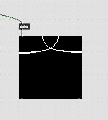
Once the cross correlation values are computed, rather than send that to all four lag maps, it takes the index as to sensor picked up the onset first (step 2 above) with the thinking being that those TDoAs would be the most accurate/correct. That then does some binary jitter stuff to get the overlapping area:

Screenshot 2024-06-09 at 3.34.40 PM

Then some more jitter stuff to find the centroid of the little overlapping area.

///////////////////////////////////////////////////////////////////////////////////////////////

So the overall idea is to ignore the furthest reading as the cross correlation isn’t as accurate (nor is onset detection).

The MLPs role is to improve non-linearities in how this approach behaves close to the edge of the drum. This lag map approach is super accurate near the middle and does quite well for a long time, it’s only the furthest hits that get a bit more jumpy/erratic. I(/we) suspect there’s some physics stuff at play near the edge since the tension of the drum changes and energy bounces/behaves differently given the circular shape etc… So the physical model, lag maps, and probably the quadratic version, can’t really account for that. At least with the level of complexity that they are generally implemented at. Nearer the center of the drum it’s just an infinite plane of vibrating membrane, that seems to behave quite predictably.

There’s also the side perk that you also wouldn’t need an accurate physical model/lap map to work from as you could strike the drum at known locations and have the NN figure out the specifics.

Yeah I misspoke. A single layer with 10 neurons.

I’ll send you the data test patches offline (will tidy the patch up a bit first).

Actually this is correct. But getting relative onset times is the hard part here - if onsets detected across all channels aren’t aligned, nothing will work (they could even be consistently wrong - but consistency is the hard part.

Note also that lag maps really are only a thing because numerical optimization (solving multilateration equations) appears to be hard to achieve within Max - that’s why I came up with the approach to pre-compute all the possible lags within a given accuracy, and index into them to get the position of a hit.

So really I’m sure that the issue here is that the onset timings aren’t aligned properly - this means that different datapoints will contradict each other, making convergence hard/impossible. I’ll discuss this with Rodrigo in person soon, so we’ll know for sure!

The 3 vs. 4 sensor thing is more interesting from a technical standpoint here, as the 4-sensor data is easier to align (3 out of the 4 are closer to the actual hit, which yields data more amenable to align with cross-correlation).

I have to ponder this a bit more later, but I think zeroing out the last sensor might work in theory, at least if we don’t use a bias (my example convergence without using a bias). Then again, 0 holds meaning in this case (same distance to sound source)…
There might be something more elegant I haven’t thought of yet - at the worst we could train several networks, one for each configuration.
In PyTorch there’s also a prototype MaskedTensor implementation which might be just the thing for this, although I haven’t used it before.

1 Like

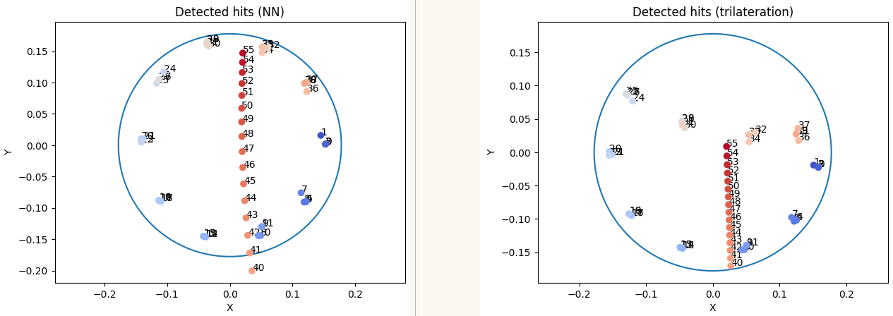
Just a little more context wrt. the nonlinearity we’re trying to solve/the motivation of using the NN - here are results of my corrected air mic data, once using a trilateration (based on calibrated microphone placements) and once based on training a NN on the same lags.
Here you can clearly see how next to the close microphone situated at the top/north end of the drum (the setup is 2 overheads and one Beta57A close) the physical model doesn’t detect hits accurately, whereas the NN solves this pretty much completely (one layer of 11 neurons):


(I had separated this into two pictures, but I’m only allowed to post one, hence this screenshot)

Note that in both cases the later hits going through the center are not real hits, but some theoretical lags I fed it to gauge interpolation performance here - the whole thing is based on just 40 hits (4 at each of the 10 drum lugs).

1 Like

I’ve still not had a chance to really burrow into this. Just to note that the shape in the right hand picture looks very suggestive of a sign-flip somewhere (which, I guess, is a built-in challenge with solving quadratics)

1 Like

Huh, thanks for the heads-up.
I know I had some issues with sign in the beginning of the project, but (at least thought that I) solved those then. However, this is already quite some time ago now, and I wouldn’t put it past myself to sneak some error back in :slight_smile:
I will double-check this just in case!

Edit: Just double-checked it. There’s no sign flip/the equations are fine.
Actually, in this specific case the calibrated mic placement is very close to there being two solutions along that particular path, with one being the correct one (at the top/towards the rim of the drum) and the other being at the bottom respectively. I think it’s a little bit of a pathological case - in principle, when fixing the z-axis, I thought that there should only be unique solutions, but I guess that with some measurement error I have come across a case where it’s easy for the optimizer to stop at and pick the wrong one (potentially because of the provided initial guess?).
In any case, thanks for pointing this out - I was lazy in not trying to understand exactly what the non-linearity here was (tbf this was the most striking case after fixing my data, leading up to this there was a bunch of noisier results that just looked like ‘hard to generally model close towards the close mic’ on this dataset).
It might help designing the calibration as well as the later optimization a bit better to prevent this from happening! That is if I don’t end up just using the NN for its ease of use.

So re-re-revisiting this topic, but more relating to the original question(s).

Specifically, taking a dataset, and wanting to computationally remove “outliers”.

Even though there’s a lot of nuance and variability in the overall concept of what an outlier is, I’d like to try doing a vanilla thing like using an IQR-like thing to remove entries from a fluid.dataset~ that do not fall within a certain range.

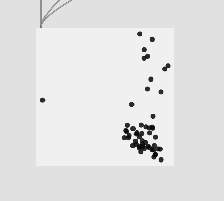
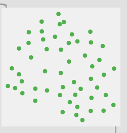
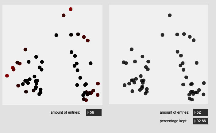
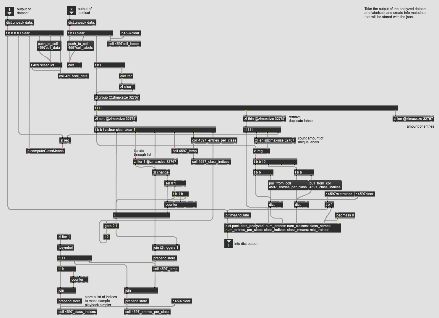
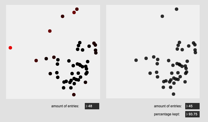
So I’ve got a test dataset I’ve created here of ~50 hits on a drum, with all of them being in the center of the drum, except one.

That looks like this (when reducing 104d of MFCC/stats to 2d with PCA):

Screenshot 2024-07-30 at 8.07.56 PM

It’s obvious there’s a nice big sore thumb sticking out on the left there.

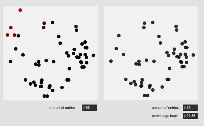
(as a funky aside, UMAP does a really good job of bending around to make the same dataset look more even/consistent):
Screenshot 2024-07-30 at 8.12.22 PM

So that leads me back to these questions from earlier in the year:

Granted, doing this in a more generalized way and/or baking model evaluation stuff into FluCoMa would be amazing, but given the tools as they exist, I’m unsure of how to (computationally) go about this.

My intuition was that using fluid.robustscale~ would kind of highlight what the boundaries are, and then pruning can happen from there, but now that I’m revisiting the idea, I’m less certain that’s the case.

So for this dataset (a single obvious outlier), the dump output of fluid.robustscale~ (after fit-ing) looks like this:

{
	"cols" : 104,
	"data_high" : [ 30.581794738769531, 13.000612258911133, 10.037630081176758, 5.3085618019104, 6.018487930297852, 2.021916389465332, 0.848324716091156, 0.765896081924438, 1.06262218952179, 1.452565789222717, 2.112335205078125, 0.862759113311768, 2.763136863708496, 12.276057243347168, 5.509377002716064, 7.957759380340576, 4.753504276275635, 5.990605354309082, 4.251277923583984, 2.937907218933105, 3.485923528671265, 2.938843488693237, 2.913998126983643, 2.774752140045166, 3.639249801635742, 3.887264013290405, 14.115323066711426, 4.69122838973999, 0.553495168685913, -0.131238982081413, 0.213149234652519, -1.938851475715637, -2.577592372894287, -2.483938217163086, -1.875616312026978, -0.850980579853058, -0.697157442569733, -2.463658332824707, -0.634175181388855, 49.340724945068359, 20.124025344848633, 22.891349792480469, 11.624850273132324, 14.796707153320312, 7.008070468902588, 5.19269323348999, 4.832007884979248, 4.893986701965332, 5.044748783111572, 6.751631736755371, 4.703028678894043, 8.506461143493652, -2.038554191589355, -1.10502827167511, -0.309468746185303, 0.122847683727741, -0.121892727911472, 0.686809778213501, 0.188267081975937, 0.112953647971153, 0.182357087731361, 0.138201996684074, 0.098457992076874, 0.144962400197983, 0.043204858899117, 12.018776893615723, 4.795723915100098, 8.32282829284668, 4.344447612762451, 6.511087417602539, 4.473029613494873, 3.787625312805176, 4.316407203674316, 4.021364212036133, 3.955054521560669, 3.870914220809937, 4.25395679473877, 4.52251148223877, -15.492919921875, -5.780171871185303, -6.724682807922363, -4.034712791442871, -5.375152587890625, -2.843552827835083, -3.433658361434937, -4.32219123840332, -3.258991241455078, -2.871530294418335, -3.366295576095581, -3.608817100524902, -3.475852012634277, 14.851345062255859, 6.138422012329102, 10.578435897827148, 7.206689834594727, 8.897109031677246, 9.495023727416992, 4.948744773864746, 6.158343315124512, 6.242160320281982, 5.219316482543945, 6.084890365600586, 6.345504283905029, 7.027889251708984 ],
	"data_low" : [ 26.191486358642578, 9.574945449829102, 6.620645523071289, 2.843806266784668, 2.807369232177734, -0.985171377658844, -1.125044822692871, -1.30290699005127, -1.20161509513855, -0.226947456598282, 0.25296676158905, -0.72233259677887, 0.531012654304504, 10.098834037780762, 4.273066520690918, 5.313149929046631, 2.820538520812988, 3.69580864906311, 2.094550848007202, 1.802595376968384, 2.119510173797607, 1.782445669174194, 1.723166942596436, 1.722331166267395, 1.927119255065918, 1.940992951393127, 8.993439674377441, 1.229231715202332, -2.125874280929565, -3.548841714859009, -3.423045635223389, -6.588680744171143, -5.418133735656738, -6.930398941040039, -5.574795722961426, -4.614691257476807, -3.475356817245483, -7.805746555328369, -3.768628120422363, 42.952033996582031, 16.204910278320312, 15.380155563354492, 7.414056777954102, 9.216808319091797, 1.834875464439392, 1.449130773544312, 2.861218690872192, 2.363692998886108, 3.201898336410522, 3.320005178451538, 2.329033136367798, 4.335367202758789, -3.612165212631226, -2.753234386444092, -1.641318321228027, -0.77306193113327, -0.695102035999298, 0.010002513416111, -0.38754665851593, -0.470703452825546, -0.165483847260475, -0.219168186187744, -0.154613390564919, -0.16433510184288, -0.179743826389313, 9.062831878662109, 3.184345722198486, 4.803331851959229, 2.746824264526367, 3.8500816822052, 2.675636768341064, 2.31768274307251, 2.744240045547485, 2.634230852127075, 2.422847509384155, 2.519099473953247, 2.670222520828247, 2.333182096481323, -23.174200057983398, -8.302213668823242, -13.476778030395508, -6.165921211242676, -11.545127868652344, -5.737985134124756, -5.956611633300781, -6.633734703063965, -5.787296772003174, -6.410497665405273, -6.020631313323975, -5.820859909057617, -6.696999549865723, 9.177730560302734, 2.429767608642578, 6.45185661315918, 3.115428924560547, 5.478538990020752, 4.147716522216797, 2.748483180999756, 3.553527355194092, 2.893657684326172, 3.111792087554932, 3.181158542633057, 2.868452310562134, 2.6861252784729 ],
	"high" : 75.0,
	"low" : 25.0,
	"median" : [ 28.130329132080078, 11.447613716125488, 8.722565650939941, 4.208566188812256, 4.727733135223389, 0.151984170079231, -0.271058887243271, 0.102985523641109, 0.033736363053322, 0.619500994682312, 1.214381337165833, 0.167311534285545, 1.852454781532288, 11.191783905029297, 4.72960376739502, 6.638882637023926, 3.630451917648315, 4.601123332977295, 2.784881591796875, 2.470267057418823, 2.75894832611084, 2.336608409881592, 2.251246213912964, 2.364418983459473, 2.599587678909302, 2.659344673156738, 11.234467506408691, 2.9806809425354, -0.482804954051971, -1.431396007537842, -1.111536264419556, -2.626004219055176, -3.690348863601685, -4.995597839355469, -3.402292728424072, -2.885841369628906, -2.108852863311768, -4.301197528839111, -1.824331164360046, 46.049915313720703, 17.679426193237305, 19.052764892578125, 8.79703426361084, 11.126683235168457, 3.956401109695435, 3.132654428482056, 3.86205530166626, 3.328060388565063, 3.939832448959351, 4.67938232421875, 3.583936452865601, 6.212700366973877, -2.886626005172729, -2.159001111984253, -0.879908323287964, -0.344644784927368, -0.378239333629608, 0.247296527028084, -0.156835407018661, 0.003652423620224, 0.006721267942339, 0.020111301913857, -0.017231771722436, -0.040211599320173, -0.049210470169783, 10.393404960632324, 4.053122997283936, 6.364108562469482, 3.656114101409912, 5.195977687835693, 3.615442991256714, 3.270465850830078, 3.38213038444519, 3.350111961364746, 3.065279722213745, 3.12665319442749, 3.214472055435181, 3.496065378189087, -18.82463264465332, -6.872976303100586, -9.52934455871582, -4.964044094085693, -8.996170043945312, -4.101149559020996, -4.604101181030273, -5.291317462921143, -5.187638759613037, -4.665089130401611, -4.567389488220215, -4.630684375762939, -4.751554489135742, 11.571628570556641, 4.017403125762939, 8.223664283752441, 5.305298805236816, 7.501986026763916, 6.138976097106934, 3.876525163650513, 4.242972850799561, 4.761866092681885, 3.802885293960571, 4.407547950744629, 4.490260124206543, 4.886268138885498 ],
	"range" : [ 4.390308380126953, 3.425666809082031, 3.416984558105469, 2.464755535125732, 3.211118698120118, 3.007087767124176, 1.973369538784027, 2.068803071975708, 2.26423728466034, 1.679513245820999, 1.859368443489075, 1.585091710090638, 2.232124209403992, 2.177223205566406, 1.236310482025146, 2.644609451293945, 1.932965755462647, 2.294796705245972, 2.156727075576782, 1.135311841964721, 1.366413354873658, 1.156397819519043, 1.190831184387207, 1.052420973777771, 1.712130546569824, 1.946271061897278, 5.121883392333984, 3.461996674537658, 2.679369449615478, 3.417602732777596, 3.636194869875908, 4.649829268455505, 2.840541362762451, 4.446460723876953, 3.699179410934448, 3.763710677623749, 2.77819937467575, 5.342088222503662, 3.134452939033508, 6.388690948486328, 3.91911506652832, 7.511194229125977, 4.210793495178223, 5.579898834228516, 5.173195004463196, 3.743562459945678, 1.970789194107056, 2.530293703079224, 1.84285044670105, 3.431626558303833, 2.373995542526245, 4.171093940734863, 1.573611021041871, 1.648206114768982, 1.331849575042724, 0.895909614861011, 0.573209308087826, 0.67680726479739, 0.575813740491867, 0.583657100796699, 0.347840934991836, 0.357370182871818, 0.253071382641793, 0.309297502040863, 0.22294868528843, 2.955945014953613, 1.611378192901612, 3.51949644088745, 1.597623348236084, 2.661005735397339, 1.797392845153809, 1.469942569732666, 1.572167158126831, 1.387133359909058, 1.532207012176514, 1.35181474685669, 1.583734273910523, 2.189329385757448, 7.681280136108398, 2.522041797637939, 6.752095222473145, 2.131208419799805, 6.169975280761719, 2.894432306289673, 2.522953271865844, 2.311543464660645, 2.528305530548096, 3.538967370986938, 2.654335737228394, 2.212042808532715, 3.221147537231446, 5.673614501953125, 3.708654403686523, 4.126579284667969, 4.09126091003418, 3.418570041656494, 5.347307205200195, 2.20026159286499, 2.60481595993042, 3.348502635955811, 2.107524394989013, 2.903731822967529, 3.477051973342896, 4.341763973236084 ]
}

As can be expected, the range is fairly narrow, given that most of the hits are nearly identical to each other. So it would follow to think that when going through each individual point in the dataset, that I the outlier would be the one where the distance from the median is greater than the range for each column…

BUT

that would take each column (in this case, MFCC coefficient and/or stat) as an “island”, independent of the overall datapoint.

So this surely has to be something that takes the whole datapoint and checks that againt an overall percentile. So I guess it’s an IQR-y but not implemented in the same way.

Now since fluid.robustscale~ isn’t throwing out any data, I guess it’s fine that each column is treated/scaled independently, and as such, I imagine the computation internally goes no further than that.

So what would be the steps to go about doing something similar but, um, “manually”?

I guess I want to know the overall percentile but as some kind of average across each point?
The multidimensionality of this kind of confuses my brain here.

Thoughts?

edit:

Here’s my test dataset:
dataset.json.zip (50.9 KB)

I’m sure there’s a ‘re-’ missing :grin:

Ok, so what you’re describing in plot is a sort of geometric idea of what an outlier is. The intuition with using robust scale to try and something out about the distribution of data is good, but these global statistics don’t give enough information to determine how a point sits with its neighbours.

It’s quite common to use k-NN for removing outliers based on this idea, but then the usual caveats about dimensions apply: what makes the curse of dimensionality cursed (ok, one thing) is that distance measures have progressively less meaning as d increases: everything is just far away. Also, these approaches can be expensive because lots of distances between points need to be taken.

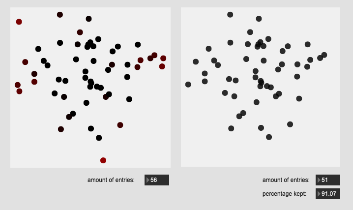
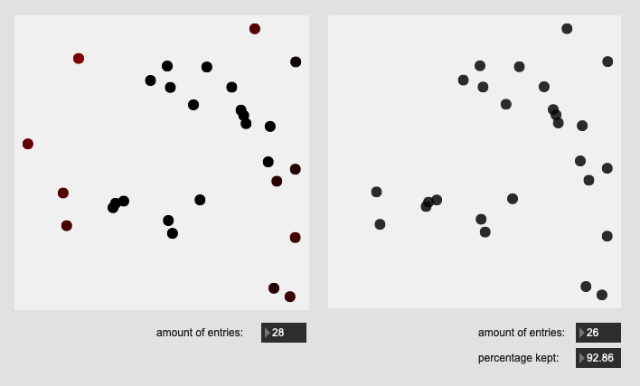
Anyway, I was curious enough last night to see if a k-NN approach could be implemented in FluCoMa and how it would do for your test problem here. What I opted for was a scheme called ‘Local Outlier Probabilities’ that we can implement around a kd-tree; it’s nice because it gives results – an outlier probability per point – on a predictable 0-1 scale, which many other k-NN based schemes don’t.

It works by trying to gauge how dense the area around each point is by doing some basic statistics on the k-nearest distances between points. Seems to work OK, even on your 104-d data


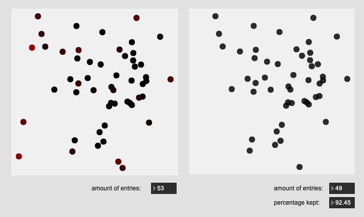
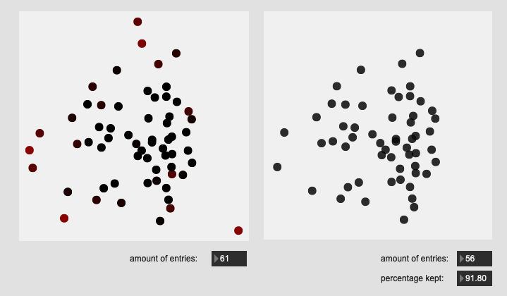
In that [multislider] is the 0-1 probaility for each point in your dataset, no other preprocessing. That 0th point is nice and clearly more outlying than the others.

Patch:


----------begin_max5_patcher----------
15640.3oc68s1biabk1ed7uhtXlZ8LiknPeA2ljMqyVopcSUa75px99IaWSA
QBIAOT.L.fdjbpje6u8EPH.xF.cSz3BkoSkQRDjDG7zm9bN845+3qdyhaSdJ
LaA3ife.7l27O9p27F9Kwdg2T72uYwiAOsZSPF+ss3wvrrf6CWbk3Z4gOkye
83cOFGFc+C2lrKMCfstBjmrILMHdUH.u+cSeSQwaBy4eUnhWbaP9pGhhu+So
gqxEjBDSfKoeEXW9OftD1OPnkVfe5kupjc46+tfEup3kxedan3KZwhxOPzZN
clb6OeMwwYA6E+me0Ww9mq54i9aQZ+7gftKsuBXSHref74+q4d7Hmzi2tM4Q
YahVGlt+4IKLm9.QeWhamEewnBURudV9yaBqRiYQ+J+uswx.EXafhkK6F3.4
2GrM+G9jFQETinxUMhLkKUaCRCdLLOL8SgwA2JdDrNATKN7Kzu4i3I90Mf6S
S1sUeNCAHX6h3+.1Ai+ofAvEl64LGbKXyhSbkl34ve75h8uwGxaChuukGTKC
9ftNZU9xn7W1an9Cawdcn3Y10rhxr8M3C4VvljUAa9D6dGQ2ZrMM41fai1Dk
+7IuFCEqtt9hM05+byP9nj3fzma.A71Sa2kDmuW7ChoxnB0QW3DvQAdPe2Qa
B+kvzL52ck6+aVDrcakW9MU9HLP7mS3eQdWU9RQwhWxt7kRC+kn8edT4qFjR
wnbJ.sKkSgKdhJm9kulDpb23cQbRQ7hzkyBRhuvESkWksMXk3CyVe2e4WPcO
thRrCGrcb4q.dd9u.5TFi6oqweNjCfV6ewjsgwQwaSCyBiyCxKn8xKuN7t.p
1gOUEfgnkRu9cETnzKxdF3j+eJMJXS4Cv8oQqShYDQsUB1Ku+1Q4nr4perq9
vveGwAak7go7FTXogKlQeH2kcaPJagpP5+9UpE4IIapeoxO2lv6xKt71n33C
Pw7jsMewTpwQs7YuMgdwGa66lekrOsKVb0OQ4Ix+TVvuTGsyC1roX2c8u9mB
hidLHOLORrDfrJunPC3CYqRS1ro1yq3J+hjqrlxiuJ7KQqyefeipxLPe6Qa2
yDsnbUdcz8gY40es7f6yp+JkFTT4k1cawd3OkG931Mzmh5uA5tinr7rGR9RV
wabOiVU.3ECcqtmtpnxZudahLqK1LpzB2F002jXRrCjIdDJLz8XMgMKnTtvx
n37E09rUjTJz6+l8ZKJDwXd3XKHipDIrQHA1Nj3vgBGe91cgQf8AQZDNvtjE
GRIunkn9ydiZKZRiwAebYZNZP6QyZP5VKRSZRpoMQAMJR0p.whEFhkv1Mq5q
Ix0rnf1EUzvzoVFE0zzh1F0z3zgVmN07zo1mNz.0sVnN0Dof1HUzHoiVoVzL
0o1o10P0tVp10T0p1plzXIWqUCZtTR6khZvjqE6P4LGJ99nq2kX7COd2F5+6
1CudShyaRjNQXOpPLBBuzUhVNIx0wGbU4Gx8phyAdzWlTUe0T+UWEXewx59G
5Xvb0lvfzVgRT2PIzV.ePKq8GnRIrD1IV1F9gf9iAB1A23OmDE2W7yl6WEBl
zr8VFG8fP2Y.5E9z1TP1eOM+cu8N36AeP76H1u8tem0mnuMp14ev5m.eC.99
9ti2Ey4N4pvAHLZT3RgPzL.myA20eIlNHNmIwSK1TTWv2caRBxUShIDNCvxc
wctmWAvr3PDPrvgTJxKpr1mNvQqY.Ndn2K6ITVn74XeYNLaqslCJetquZdDh
DQd3BnCYHUOh8zsCfdy..7wvfduSFZAE3lXuL1WQFP0ELdnCTNFKmC5x+..t
r2VRVfkPgahMmsPpvP5LGLHuLvs8GCINio8jV1ulzoTBhirVE7bPnXvSQOt6
QfUu2NKrXD6yC13wILwfKXziLCfyaLfbwBfjPFaohdyAFxsfvz6LyoWvhbX.
iM094tgPW2Exnt5t0+XDpU262lK9k7U0jq9awc+s6xe0b6eat9+H2+qXH.NH
L.DgylvBem3K7NN10+3E1liEfhwCP0XBnTbAzH1.cDe.0iQfBwIPoXEnT7BT
HlApE2.khcfhwOP0XHnabD5HVBJEOgtioP2wUn6XKzY7EZKFCMGmgVh0fxwa
PiXNzbbGjI7Sl1HouuCzJIj0ejDsNz8znEkEIVFRbJQq8+6QaQOVIjkj2QUG
gaIiFWk73igwxWD4eAwqCeRhP4CTxerhdSBwRU7WW4+8gwFdI.52wAi51N.c
rE3Hi7sWzD4drMAxAwNsMnK6CZ3qsM6D5vVgtsWPcaF5xtAo1Nzj8Cqy1tTN
OTyoSfmHQWwtx4MZ2TBMLmPGSJT1rBMMsPAyKzyDCEMyPYSMT1bCEM4PcyNT
1zCML+PGSPNEyPTvTDkMGQMSRTyrD0LMQIyS5xDk1MSoCSUzxbEMMYocyVZR
lbS5Va78qpN1CRXvX.ro2TMksVM7lZNxLBuV30zQtUWkqhtTq6rsnQScjaty
PszrhpiSx4aU0FmxDLuTB+e3uRkix08s9OtP80IBpRDzrKRXajeuWp5RM0ou
bhWzxsrCsnBqiWKPreL8GiCSu6cO89+A6WY+e.8+Bff+c.U.Exl3g7s8Q+dP
wEPzKbM8BdDhuiK1o7BX1m.tjffDH1k.Ku.g8InWvFCsQVH2xKXK9DVNPhkM
A4u+BaAhaNF4Z6CYeQETUVz8wzKU9UGcG3cOA9C.q2u+RWWdsmn+UvsYzGrW
974rO7RqadGqfo9Fv1OT8hOKtH3Zv6X+Wf8Gxoum.x6+P96Y+B98hW.U7SH8
meH7osu65mXeObzKOMjZYWrfZ9.3Yw29+bOxRWqY3JCuihgz68bbSohxKoOK
JJvDp9FQnqiHbC1smHUpePwC23PzAxkaa2lnXc0fweTYeN8VWxR1ktZubghs
8flACpgC4QwkVa+C6eh4elAgSyTOWvS34Bq8ykj27wuyQ7z+6cQQaG+mZR81
rOdyMe4KeY4Om7P75UIIedI8SdysaRt+FpQq92XAuA5eC8HBwquNXSRb30go
oIoWe2tXdYZQ+y6tQ1cgsxsJYmvKIXC4kAhGTjL5hSHUF+v96nG3wadmYqVR
Uc1fhyFTa1fRyFTYJUgIUYC+k+cf+F8TRf7GBEJjRtC7TcEokpQ4ZQ+n3Oq7
FtFdnxzW9t+Sf+MveC3tDtD4zn50dnZkd1rGVVpec+8shB1O7bm7zPOyxTCs
31FRD+fmJfFfsFMkr0bnnSOLZomGFs02IuFzCi3yV+AqhLl+z1soIOwccA39
fczSeGDC3B7A6E3C5biAxTtTVjYHh7nqPXOK3xFvq9pro33360nwYGuD0lwK
RVnT2XrFLXg43aYVrbR7W8k32SLJS8rnrnH0eva5PWUuf46t0eR36yOEjmmF
c6tbwpVa4CPuBa28aRtMXyANnpsn68UM+PNPYAhLIwsJEtEWN41t7Wil0VX2
CC.WaBaaPP6.goRigo9YXsHdHVNZgpVsAYXiCY0qGRoxAqijMIB4.7T5g0PG
8r2fTCn+whMTdstOTHTQJjkygSCEZoLENEXHeWs5z3DPgdXMHPVVnM5T39ap
RTnGYJ3CsvZwIZOIznsVzniz2cR5ZQ5E.m8DOrYh2ZjIdGsHd2Ig6vUKZzS.
viLM5qCMBslBbjeWUVqIDNIzndZ18lLZTYg93IaoVc1woXacogi5I54f28iQ
q2lDEmWXILzAKJUMKQG9AZIZ6Ar+brMdgn8Rv3K0xSKZDMIrxHc2sM5vHTGE
T7SF1ALV4hU8shJ9U4ez21rR29QQlOTd4AXXayU75eqZS9r0i62r+SbwNh1d
Ze6zURZThG4K.GuQqIfEmj9XvlnrPv5v3rn7HJ2QuZIX1NtKs7cgNdVh+CBY
sSF3v0gvbbuzgvtzgvtzgvtzgvtzgvZqCgYltJhiM2PYGi0sa5t4r7ZooVYw
gLa3H1DB78ek0efXGXa76OP9dyhh9tb1MH0XsShoz2QrcFuuq+MZUAtuykp.
evpBbgodDQtXznodsZtmhl7opYeJY5mFl+0gIfpaFnBlBpj4fJYRnBlEplog
JYdnhlHppYh5ZpXGlKpjIica1X2lN1s4i8OaR9sSQf2bEJeJoKFWxT01UmIK
+3NyKPm4d5CugtryxR2+9tvzi01exntuHgr4MlMwL+.YjBu2dtimYg4fJdfy
PvIxSnf0xz3I9USd.ivduT.OlOMf6tGCzqL.FMu6HDRZZimLubQaXUHgn4V2
X2mzusyEzPmJ6Hwy9Kl2.e0AqkgPdQmVPqVwgR.+QSgqFAcuYNnevTaS4i+1
AGusm7Y4VeAd0.c2oDzk2BNqi5G0FNOY71i6AQDbf54Lci0NybFb5wsomubM
3dy0qkDkOKT31LW73anMYli4RZQp8ErEc+Xj83C13YNXyr.2TRSJ.agCuJbw
tZfMQEvt5gEZwYwGsDH0dSEKyE4n7aVD93sszVbjNqTa+M9Xv1s0Fqpsyyb1
d3C6JGOaBN6gO4rs7CMaG+qnZ.QVltg+4aO3H7jVXgN9ZVad9yoJKzmnI063
MindGWcod+4D06IK+nai5wyMpWKr2cNQ8Nm0TutUyrCYNQ8ZKyANmndnt6Zc
lSUR9o.8vKER9jkYIWahAxfvwYECR9wbfL37ZYjVHZnL9nk9VHOLzW7ed9zy
0RFO7zcNLd990MfrMQqBAHCj0c7LahGICaaSMwU5LkwbPWlnb8K2EsGkbWzf
8XitZj8lsGabTRk8pqGavclGFiMVO1vw47tGanZct56LAU0F1gLyaOD5TFt1
SQG1vVmJb0YJptRWsJtRmIfB80oAEvebF6MJNHc2JO5XnmFTn6TvG5nCen+T
T0+d5vG56OA7g9d5RgiNenNxCwNNWpS5CoUMpD3UIwY4oA0JTmFOskzT7Cxq
kDL0tMhmCF4Vb.Vauq.NtCX8+huT+uJU+u19hCw4bo9ee4cco9euT+uu5q+2
Uah115wwwcebbwbhE5ZuzFhcbgdrFkCwZTbED1dNLO2YY6ajg7jFxqJLhLV0
TuOMe6ZPPismCtMOBfr68zcmZ1gXvjSsw3DfzN4L6FJsOybTI1eYQrEbI7e3
Lhtsb91ZfMBBCQB1wIEigmDFiNabMrPWDx1spPTy3hXz4qKhYxzU2uMLcp71
17H6kXc5zfhmnQuQGaqU+YaRbDK1ApENZOEQDv1VKZzcRVqczFGu3ioSyGST
6m6QS3ytX75HLpqeNShakbiNTh3NRseuecCHM79S0eaEXhn1iwdJfInVcv1U
s4jMhiIwjiK3rW.EJIW1max.uE1S2QRrJlSSdCmGHI3Qhg4ZvICGTEFb1khe
H8zQ5fFGdpnZ.BFYR.43B6+EDI31cYzGTvOjy7czOABx.4IfcYgreK.vjAtF
Po0v6qkDLMN6izRpDwRjOQ9jVF1QMa7YMHC4OVavr5wlJp4aB1mhIh6vsmBM
VBgY9FiZZDtQHAq1FKTK4FkgfD6QBRRoDUH3tHpQJAwY2kj9HntT47jMgzKs
JrQPinhtq8s7EkTdQ5T40UcoDCQFI.jKLB7sLoOfem0mnuLU9E3aYgjfxp8s
Tn69vV33TaSHlM.wOrS6hj2xFzwP.lj8q5xFITMQHLGdGtNJWDCrph3jUyhK
Du0pNMwpZ9Ehq7iZDfllPKsdIWTZVb4BSM6i6pLJap7IqEUF156gtUuYPhdo
hXUgFFaxaSAJNcMXK8M9QV.f+kvzbl9ysozyQbazFdKFjp9D7CVWC+oS03cV
GG1trEZib8j0fbTSMIhPFKKKPw6AlRAeOjjr95xNl8ZdWXbIfcRQVLuxLt8E
E.mCKhsGsQW.iml0FHyZwZavHLKu.F2Ee.zEk+7KfGHfh2e22cxcebHhmi7D
eWCvjgFKawn5X6g0XEZQcgMOazMhkGHh0Xo3DjQ+e8zMAPgcoDU547XUrpnU
UgTqWFIv4tM6hVu7yqySCC+WL6JXho+DipiBMtrmBuKXgjzM+sJ6kWChyFPX
6Qa9GrNHOHKLGcPKo3DfJLjelHO7f5HFDlbIamzOam7rDcBWL5R1NcIamtjs
Sm2Y6j7N8Y0t7I0VRpbUP9Cg.9gtyR.eIDrJHFrNg9GzikeaPVzJ1AcXhkXS
H86RRAe4gv3Cb0webuJB9Wzg2xZpZs6YTsQHwPZVzWVKbmnKoOwyFhWb1DTe
XQOmrnSgZfn4Cmu4AQGIFkvCbx33zN8n7KxUhVleUmRhl08X6vZtT.rTw7Aq
9Lee7GMS56gDcoSe+QI6GmCC.EAC45cOt0LEj8d9Q+QieDg7lE4PJCCEJkLz
D4QH1z0wTSDEwhLP3TxtQ04Pl4tuiYlFdW+q0ce68YnqiGzCZWTFKN9ziQ.G
kM7HzbH4bEtanv5m+kgx6Yge47rFws8maYmaW8oPyxpgQu9ai.l0pRDFeF2F
AzaPOOEy4YjsVy44IgDc0HQaKefl.ZDoLMNEIZKW3ixK0hmnoAGsl4q0duhZ
8Fb4qS.F5bFrNaqkbGuKIqbOBMTFycgu3IvSMHs7R8iZUmsn9IsFtDDCBctD
anSXRX64IFrs9WhMzkXCcI1Pm2wFpCmZD9z1Tv6d6cPvMf2dG58fO.dWYh.9
CV+D3a.v22WWbh83t0jXW1QOGCuFMJsKwtB81+UZvs7vt80TYBwqCRWCVGw9
0UgeMODaAfsIQw4r3uEtFjDChxy.e95Wzy96AAaxR.2y9h9K+4L1zOr5kuh+
sv34RGzfwgK7QkM1XAiad3+YCLI38JFcSVZMIyMPOUctDHDVBMVONw8Vjgn0
zJ7kOT4NrZ+wzyGuiV.QhDbejbOJ4bM.x+LUHK.22d9BwQz0j4x.8FmncNKZ
0Kk8eZXe2XiDUqJVrkdDa.01jw.GkO5.eAH+bbX.8XR4f216N4MTL3.ghL71
cbBEGw+UR2k2yVzt2PZoy1.8SdxbX+7G.XSgfEagGSDbdLgCrLEBhKpH6wDB
smAPnjwzr9IImKWHXg5DrwRelVmKy0PRxL.I+E9w3Ymh+Cr+0Lmmo.S8bFGE
K3YhYN6dzLaqwtDwt6QyBGr0rIw31alCyWGk+Qes9tfSrXtvXiMUBd03TLsV
VN3OaRAoMTPEc6t6Ly1bnivUNFyobTJik0YsmkMupNSSQtbIJytQ7HMHzrgm
TdU3A915EO.z1PtZCWTUqnwCqgWleQ8LssmUG.mqYp+GBuPFp3L39iS2+EQt
jAmsUjKu1GDTDgdFer4pKH6y2L3TmYhgs6Tz1G0IESmhwJBgnIAN1HHQmTQi
LEYEIQmbzkLI4VpVyRqoXDFoQp7QHSDAp7R7Tjxl5vChjmApOFslmNBY66rV
ECZUdFg4aW9Gi81KcjwOEatzJedmDY79m.yw3hgj4NEB0hBQSRBQqS9POIoU
NVGLTNfmjtVjFuvwcKjNjN1ZtCtMHQnDbsFeySTky0dJT+yuoPcNnAZJ18q0
QgFcInZIBENIKytZUPfW5+8GQq5z+6qk6kmPSFyov2kpz9tQc1A7aqQiAsPK
NafEaosB2w.jfiDHw8D98oI611SFHY8RTGXeqIIF4Q2oFj9biXkO9LCpJZkn
iB3P7Ne1rULQE7c6aiNrysWXi1C3OzA+M5b+1dza1EzloGu6V0yzM4UZIdj1
.3yQNqWWdCVxy.8TFgZZRH35zaHn7tdri3eAUjYwTErQxHW5nprtoCC4dfCE
ac0Qa5v0VU5.QFP5vGqHYvLkX3Hixu8tgCGuAmNfJwdPFT1Cxr.OHdJyd.Gz
kEnhzgOdvICk3NbbGRtCG24.bvaiwJBGCIcHjPpNc.GrkEUElhICJdbbnGaz
apjAk+PYcbjAc6BwUY5XP04STVYKzYH4SQJutfGRk9XrxJ8QCJ+ARY9CDbPU
5qnXLA6wvJVWMSjGZzPEpfLnFDBclCjAa3cnpHc6gDNTdih8fqvGoxNkAceh
mplcPFRw4B5PIdCh0fupnFOp2futzOtihWberO5JtGEjSiw6PVrN5HNGGFiC
Aww+WAHwumU7JjfFZqQe7hCD++ReF7kn7G.OWosGH0SQRKeMHTTxZE0.XQyf
thihj6jn50xmvsfZ9.Uyon08VrzmBTyOEthNFksmnltsNLNCxmbgs5XXYyuv
5Oz6KleUYnNZ5205nsqowZ2oy.UOwzq1qlih0FwcDsZcGnk74Npbmu1hiWqi
snEF7Ar1byLMYcltOrPjnIwgc8KRCMy9zZYvsOhxeKMLX8I+TJ5RRN3NdJQM
9T13dFhIETTucX27BqBR+vHqF5EfF3Y1wj7xrEVvOt3uFrhtoMI6Av+8e9i2
7+KKLM6ljuDFeyeN4KwaRBVmcSAvr7myRh+wEZyLrWufin7lQVlkmun9u0DU
Xv.U1Zdx9x1dwCQ0CEQkwE49WYS38Aqdl85qR1HZEhv13SNt29A9OS1TtcRV
nVDswOWK+8JOaUEZQ8fx1pFuVnRvormws316KIS5x.6qxZIU+F8r.rei3ZY6
4cE6Bke6MVOoUKc7E0.fef9UgI9Vnqj7KU+tqUfzdufAMp3ZQz8wITnYSzpO
eHpV11EohVF3Ue33s5ivh43t+RJ54ggEim.O+WwrBnokSnIag+tjbPzia2Dx
tZ35q.T1EPR7Jwryl2d6BAqR1sYMehzm+PDe5zmy5GNTsLfnX52La50yDdJx
Ccd2sSTLooWGSkJyl9tzm2G4MBOVi0KIM5d54Q1rgdS1vuKrOcI+W0dfGVS8
S1DwTsQzwhPN6KVRMrMGeRpbaBf+OYzH+4LjZ038+G.ppm8yiq+9tvzmWB99
MAEGHI+gzvrGnadVtb4BsexwhVAaQa0vQwikTsysBkytWrQxB56X45QvPrKx
1V5K0njPaiawVkI4i5Fg6wE8PEHHez8zeiWvvS4A8my1Eo6yhsn0o3IX4QVd
k+njvXMH4RQyBq+1tIgtiKkZjyh97He6KIcrLPvpUocliSHuYtfN1pvll2Nt
h1Z8oZnF+dKWZu+vY1dgn0OIjoDt9Te58EcPZ6AXSPwbpxPVvuZSXP5UExPA
Vf+.SU9UfxSnxaTf6QEVqLHCrIYUvlOs+03ZqTB1PcCaBSVIHhYMuGYOTbLb
sL+qSkKQLBpgPqAfKAO7aR3rCmppTw.dSRaqw.O6VF1AfKeY.ARsWaS1GgmB
CNuH0Ec4eD7jEKdbxhV6YGZRgi6maZrivepqyHwgQ8M6NZnmIsi7uwF2dT6m
KaMKOjjrlap8igAY6X1VJj5AVGFmEkSsq7+Nfaq9sgfvmCu9Vp81gr4KG8mO
+Qlc3ogecFH.j8kP1ngcK8j.ruN1DU348VntD7+kj.xdj9YtBDPg4mS180T6
1yBCAecwdrruV7Y9B6aD7taCWEvNpPD8qKJdMSVbN2xe92Rc5O68Tw3zavsQ
2y+12FlxDnyZ01fr7fzb9Cv5v6SCVGJ87AN6WcqLHC9jz2gpLEthrkFaI7It
v0dd5cDBnsIW5KFgBZKFyCKN9SQCO4jBTQQGfwPOI+E5YLumpCmUZCzSABve
D7PxW.ecdxlPp177uFDr49DPD+HiqYlMReRYb1UON4Rv6xRRESFY5CvszuOF
2U950g+Bme4uuKXSzcOCnr+Eet2ajyV5hEM+QK2JbFZd3RHxr34J594Ll2qW
KNpM+XjEO0rQC8sA2FsgJMPJ.fzD.vh1jmCoZjuvX8..KSZZXAiCUbwa0Vem
in0PSD6RbMbHJrNIo+B948OILl+G28XmdfqkGNKTQ78TyBFJwr+NhaynFdcO
H+410zG8qo0958orSd8GWLdDJN+r4X.rMJC.5zX.vhfRX2Ky2aY0Fa5U6lD0
UMjjerbf1GEeEU1W9tzXlkLLCOER.YScCVPfoF7PUHHQdHSAC8q69Pf00PoB
GI5JbzQ.3NdhVzH+7gNml+2pAwVlTiw8gwTAl4gf6oFokEEDCVsgMMm4nV.3
1cwqdfoNcuscfVUbzrUW5xtJzrT1nPOAMKXeiZucdZzuvBkgv2AwLyQyiVUy
Q0JyYfIUBL3IYGF12vNkd+jqYuq+4Kgffb.3g77sYe7latmxQr61kzuha9kU
PhOJ3lu+4uKgZDuYLl.5VsEZKZKj5thaRelrs5Ng8r+KNovOTb1AHz0npTv9
3ZAU6kAi29DlogAhmrgg29bHSxPvSx.vS9vuq8AemrgdWY4z2wvtqxftypH3
CL6NEslPupEkmzIbWGS2ttlrcsNU6TXh10vzrq6IYWKSwtVmfcsN85ZYx009
Tqq0IVWGSqttlTcpNk5ZXB005zoq4ISWySktlmHc5kViGME5jLA55b5yovjm
63oNmQGbnwLuvrgwp1qZoEhoGU9vR02ENXiOTrE5x3CUowGpHpOPKmFEr1nv
UEDvphP1NEzpnv1VD3plP2ND71ov2NE.2gP3tED2ovXEDHqhPYcDL2hv4NEP
2tP51ET2tv5Suu67Ze7gp8TZoX.fhwUZ63CeCGe1LNLp5uAyLrAvD3Rxg46l
u+30N78mCCgIlSY3gq6v.zal9iOx0ZoCzk3PrcQPeHByx2Ox3L9ZQ9yA9WIQ
D8jAUA6ITXef63L8DgdtyhoL68gbKN5+rls1javwaz1vC8lCa3o5JyxixYxT
4vo4ErhP9KQXhOc6Ggf8PDWWlIdtiHPCmMS0kxSt8uLCaK1xi4KK+walXAc8
lMn497IxPh.DQh2yZDwRmeiO3QZny0crmCrdkOBRJfWD9XiPMw.IAaAOeGHI
LSi0oQQOEsxbNGp5s4VuoXfPvDcqSW0eRnQO857+SRi02WGZrD0G40ZcF+Gk
n9HuV6nENNM7itmAzndq0tWZw18H3KLug7oJIZvoF7k1Nvoga9uHKuKAdQo.
u3HB+EFIR+Arv0Tt1vKgd4RnWtD5kWigdoTz92v5XH80mWvBA59B4HFymrUq
2cYh3smE919vLy5jONLRTBvHWd9mYNmEd2ljfbleYD+RqH5Q7BRzadLf0p9y
1zgJ4qpIcosnOsccppoWsMcqGoeUQcr5k1XcplUQUspptUIUtZn1sCUupq9U
AUvJoFVIUwJnNVMUxJoVVQUyppdVWUzcnlVIU0cqttaU1cq1tSU2so9tYU3s
nFWYU4ZnNuYU5xD7ISwjz2mJJnpqj5Z.Yor2PaZ5aTa+9PbIp4LoyCH0z32l
5Joea0Z9TKN750z+erM.iLjeCUdqmwAcQwS0rIVCLnaOyA8zf30IOBfVHhr2
mrpCn+KMXdaI.Jpb6hpFv1bKMxrB9nEFmY9BiIE.43HD4Lsxerl4HNalTcam
PNTMH2FUw8cXjFRePp.46mYU0ppuFQd3uoj7WvsOwB9QWD72jOsmT493obcQ
VNVzYdVztHltx0hAELck8rzRJCzRZCLxqDRyGiSVZuPjCVTGjZsVX0AB6cAg
qZN+P.w98BhQJ.wG6rFo4Aibzuo381vZvwC.Moy94VB869ITtQ3c5M0aoK06
MmndWcod3bh5gxRXf1ndm4F0qE1imSTustTOYNQ8N5R81yIpGqK0ilSTORWp
2RYp+f2zgg3QkL+QVrv5kaq6NSfZJafN9gbpJSkic7f905WwnrQDYYLxTwBs
UOMTuvolAwVl2FYwshkXEhqLgChDh6KmvZ3K7LuYQr422Sg5K+HlvsTG5I5g
RSQr4Q1WhM+fEadw5ZgTGGQhr3xZeVWBO+kvyeI77WBO+vGqFvcFKZMEIasv
DJrsFwL.qc3ZtR0XHL2CayG.PyEtdQ3.Ht1SYLJgjeCA4htaIwAOoHNdli3q
RxLkTFjvlIBRj7utSSjIgy8HSlEEaLDGgph3jIBwm6BxCeZaJH6uml+tqQfO
.1D+t2dG78um9qu8NjwD2XsuApxiArw496dYv5bXYfPQ8.pPm2YIvenw1KH5
BTHauFFMHC9Bf+4.9KxKh2Y8i+3U7ji38fa3+booWGDSc0hdL8ntNfurN7Re
mY5VFPudxDEqgLSTTSIKBdISIpXVusikoSTBD9BBW8rp1NdFGhIutyEEnt4h
BZNEUantwEFMmxn.cI94TV.4qIsCaNF3uLySOOexfc+jAmG6VzM+a3aufyk8
55lEEbQayEpGoM1OmDypqT1YFsqSFyMmTP.sNEV9yBor5+ngOWDypsbJqY11
EjtDO7RppMY4GzteMBXf1ehsWEeuPfJlaPXsxUsq5tcnfrNaZrpE40mXjeXt
NqZmY0Gz8UdKUEZiXmh2wBqEx1RWTE5LagrN1cKcFjCP8e6NGhsEMnGXygga
f5KvP6wXaNU8QdRb+SiWNGnXtDWfTjQXet2woJYCyBzY.K58oI61ZnM91hPD
6.GYlRmWOYKseQp6XMhYKs8rX7RDArVh6clRKFsnvhg8qwlsDLqeTJOoIKlG
FVZhFqmHSOfV16mq6Sikks1m8FsVhNzVmtR7TzTh0p0NaOADnNH3T.frZbP4
l5rs331iOAZoAABGaBzatuD6OyIPhlqvSA8o5VDzTPfRcCVSUq4DQeJCf9S.
ApyV3IYFF3NyIP9plxKwVSghXKcnPuIPSmsNy1ENEN5p5rzPPSCONxiryLiz
gsS5vwku.pKewkwtwaZdrabn6zazU5mVlJpyP03HupUKKa8qlQhM4CXI9+0.
XzQtF+DF8HHn+wy8ckvLql.DTuAjx65wGa9ELR1F0JHkDYKGY+PiSMrCR1fV
WqzkNvGOwnZTCr2PRGVHUwC+lwihWbuHptDOUPPMJVRlHoNDGcnnHAww+WAL
wumU1RIngV7aU0FkfGXaRTbdFUqzAyy.oa1j64TnHCR44pKDdz74TtvnVbUZ
88a6cm1g88f8XcC84.Y82f87KR5mAR5iAx6eAs22Bj0uBJ0u0Q+IP8YFfzlQ
PGMgftZ9.s1zATnYCzPSFn6lKPKMUfVal.s1DAZo4AzdSCn0lEPGMIftZN.p
1T.ZnY.zZS.n4h+u4h9u4h8WOAXGUT+RJl+NKheEJd+iKZecMoftyKK39Poi
6rpiCZ9jOyq8YCeit0WZ8LvCSGpngJ6C66jPqYC1rdIPHC63gKMgMIsaXHZe
BfClYP1glp46q.RgZEotpEzhM3OGGz5vYhM3ao3CcGGh9KAOQ+EuS0P2BVKO
QeQ2xYPArpiD6gEvjlFGnSkEqn2XH5nXMT1nldRD5NV7VTU9TciqohqBV2yI
0nntqb8GL4SHW7ntia+bSWHQumniPtMDZMrBkbQi3dLwP9zC7sgOda3Z.rm6
vDyJ.HxVAHhn3NrqJ.rVAMmZKt7gVZC9LxRbGtFcE3559hcAr3RviuDpxkp6
BuE3BaaOz2dKHMcA6hiNcnyfW3T.lT0g0ufawsmT2kv8w2Y7E7iFqhRSYJ4u
gGoGw53rp52l9Iyy6L0OYByGHrSBZT+j44OS8SlKVU+S4Nj9IC45nLcfGR5v
wSY5vYPwCzgwFqQ+WRFT+FRTDONZZ2aT5n7au60E+gbcgKYSM5vYHwixmxt4
O77es6O28hSOzgt+OI+ue+GA+OL2V.9eEts.78oTx41nMQ4QgkN2U1jwQYO9
BEYjnUohiq.zSe1j+dsj3TWu8M01EU8FIld10S.Lp6TmW.ie+OlxNZ8lfcwq
d31zjujQQi2BUGBPMCAhIxDT3dBHx+vo.T+74sm3LRFBGdHOea1Gu4lu7kur
b8sYKitKZ4lG2sbc3Me+ta2D8Y9Fnv3a99fsgoY2vXhnGDze4102s3zvEQhn
iOtnn5It.WXvMKYgg.cC1At5iGrXafNb9t9KLY7ap6gxska0eV6GLwyTQgDf
bOYNZIdFoN.3JaqOuHQ9MWXdDsRQriun6hyEq544eIROWhzykH8zuH8zhWuh
pUsPZ4jKlTRVPtcEh9k1tY0wmBGVAFxq9hA16wfLpNjvS1+AE8Ne91caqgKv
VtUaqTxFBBU8sUKC+flF7AUy.tFF3AMLrCZdPGz8PNnoAbPsR8WgAaPiC0.Y
4OPiZVTP6hJZX5TKihZZZQaiZZb5PqSmZd5T6SGZf5VKTmZhTPajJZjzQqTK
Zl5T6T6ZnZWKU6ZpN878T5PGngANfRCa.EGz.xGx.CZsbtg9+58TXhHrGUHF
AgW5Zal5ObePb5teMLF0x4w4BRcvb0lvfz920.Dv29Yns83LElfykwXUewuh
wCrn3hat89aTzCBcmAn2KsybVaLG7AwuiX+169cVeh91nZm+AqeB7M.3666N
dWQeCQ3KOjxycs9hynYQ8ueW+kXVjCNhItlxropOlv5VhIDNGp+83N2yq.Xt
Oy8wlsuJIMEBNFGsVLS5OHziMjZFnrP4ixMRfdts1ZNn74t9p4QHRD4gKfNj
gT8zcmr.ZMGFhhOF1+wmHaVTwwMwdYruwmehc1BKrlC5xkLviz2RxBrDJbSr
4rEREFRm4fA4uEYLLTzkZFK6IsreMoSoDDGYsJ34fPwfmhdb2i.qductHm28
4YssKYzEL5MG5WR2X.4hE.IgL1RE8vyhQcbX5cl4zKXw.g.iM094tgPW2Ky1
3Aa1FSDNapnwr4K7NN10+xvM9xvM9xvM9xvMtIsQReeC6nHxqnn0vZO6s5ZT
DYc1NsmTXDyceXrgWBf9cbvntsCPGaANxHe6EMQtGaSfbPrSaC5x9fF9ZayN
gNrUna6ET2lgtraPpsCMY+v5rsKkyC0b5D3IlZXXW47FsaJgFlSniIEJaVgl
lVnf4E5YhghlYnroFJatghlbntYGJa5gFleniIHmhYHJXJhxlinlIIpYVhZl
lnj4IcYhR6lozgoJZYthllrztYKMIStIcqM99UUG6AILXL.1zapqIMZGQlQ3
0Bu1FaqpoxUQWp0c1VznoNxM2YnVZVQ0wI47spZiSYBlWJg+O7WoxQ459V+G
Wn95DAUIBZ1EIrMxu2KUcol5zWNwKZ4V1gVTg0wqEH1Ol9iwgo28tmd++f8q
r+Of9eAPv+Nf04JrIdHeaezuGTbAD8BWSufGg363hcJu.l8IfKIHHAhcIvxK
PXeB5ErwPajExs7B1hOgkCjXYSP96uvVf3liQt19P1WTAUkEceL8Rke0Q2Ad
2Sf+.v586uz0kW6I5eEbaF8A6kOeN6Cuz5l2Q+Gv2.19gpW7YwEAWCdG6+Br
+PN88DPd+GxeO6WvuW7BnheBo+7CgOs8cW+D66gid4ogTK6hETyG.OK91+m6
QV5ZMCWY3cTLjdumiaJUTdI8YQQAlP02HBccDgavt8DoR8CJd3FGhNPtba6Z
bJz17JRaSerVVWTefCt2vA0GbeFgSyTOW3S34hn8ykj27wuyQ7z+0qYM4ayp
VWe+bxCwqWkj74kzO4M2tI49anFs5eiE7Fn+MziHDu95fMIwgWGllljd8c6h
4koE8Ou6FY2kZUGI1PdYf3AEIit3DRkwOr+N5ARVLyWsjp5rAEmMn1rAklMn
xTpBSpxF9K+6.+M5oj.4ODJTHkbG3o5JRKUix0h9QweV4MbM7Pkou7c+m.+a
f+FvcIbIxoQ0q8P0J8rYOrrT+596aEEre34N4ogdlkoFZQDcajhwckmQXqQS
IasrY9mRG5oMOLZquSdMnGFwms9CVEYL+osaSSdh65Bv8A6nm9NHFvE3C1Kv
Gz4FCjoborHyPD4QWgvdVvkMfW8WnznS8n3o0jwYCvHg0V2w+7bZf1h0cZ7Z
qLweYf1dRYAhQl9pEtbx0rCe0VSvCrq0q7Iupn.UrEscSSL3UwtXiCYi2rZS
qYDC1EOEiwFHRCZzCOAi3DnkVyBHHZJlVQDsHQ2oXRw.0YniwRUbYu6GiVK5
Q96mg0XQNsaIZE.PKQ8Qx9yQmS1R60fwe2FT2caSCIBUlMwaRnQclbTkf9HK
0RqsaPqIgF0ZHlY4MIR+cNEwViLMp0TYk+DAmKigqSg3mMChKVgPnCwOEiBR
Wc1j4MECCROc.Q2oXGF+nSy64AoV7g9y7Q9Y49pY6PSszb1KiUuScdRbeZxt
s8aH.3h4G02YLFgDXGuQqIfULZRxBAqCiyp1rX0FnJZkjNtG2RwMvn2nEzx8
RGB6RGB6RGB6RGB6RGBqsNDlY5pHN1b+e4XrtcS2MmkWKM0JKwvfCNhMg.e+
WY8GHleXG+9Cju2rnnuiCoh6ukdXBoFqcRLk9Nhsy38c8uQqJvYC1gKUA9.U
E3BS8HhbwnQS8Z0bOEM4SUy9TxzOML+qCS.U2LPELETIyAUxjPELKTMSCUx7
PEMQTUyD00TwNLWTISF61rwtMcrayG6e1j7amh.u4JT9TRWrWF40EEaiIK+3
NyKPm4d5CugtryxR2+9tvzi01exntXhVJZ3uES8SiT381yc7LKLGTcDSZF3D
4UYjCZR7D+pIOfQXuWJfGymFvc2iA5UF.il2cDBIMswSlWtnMrJjPzbqar6S
5214BZnSkcj3Y+EyafOGbKXiYQdQmVPqVwgR.OuWBekJ5D8l4f9utAbX.cT5
3ucvwayEPYCMMGuZft6TB5xaAm0Q8iZCmmLd6w8fHBNP8bltwZmYNC99A698
lqWKIJeVnvsYt3w2PaxLGykzhT6KXK59wH6wGrwybvlYAtojlT.1BGdU3hc0
.ahJfsByidoKARs2TwxbQNJWYxsKsMpz0DbWxaT9jbuQdly1Cez8DgeP2O5S
NaK+Py1w+JpFPjkoa3e91CNBOsEVnlklmC73DX9j4b5Kw6HMe7Zi5clQUEoC
4Tv9YC0qaQc5PlSTuitTu6bh58N6ods10hmSTuqtXu+Lh580Vli2bB680j58
uTH4SalkbsIFHCBGmAE9yYLGHCNuVFoEhFJiOZouExCC8E+mmO8bsjwCOcmC
imuecCHaSzpP.x.YcGOyl3Qxv11TSbkNSYLGzkIJW+xcQ6QI2EMXO1nqFYuY
6wFGkTYu55wFbm4gwXi0iMbbNe6wF95Tk0XYGgdvqpMecZeE9SQkA54nKEN1
UAtiNcoDeuoZUV0xqzcJ5QIbLTUJzeR1onCenKZB3Cc0pa4LEXnsNBDcPy7J
k1dJDGhcHmAEatV6jgWpS5SrRfWkDmkmFTqPcZ7zVRSwOHuVRvT61HdNXjaw
AXs8tB33Nf0+K9R8+pT8+Z6KNDmyk5+8k20k5+8R8+9pu9eWsIZaqGGG28ww
EyIVnq8RaH1wE5w5+cDqQwUPX64v7bmksuQFxSZHupvHxXUS89z7sqAAM1dN
317H.xt2S2cpYGhASN0FiS.R6jyranz9LyQkX+kEwVvkv+gyH51x4aqA1HHL
DIXGmTLFdRXL5rw0vBcQHa2pBQMiKhQmutHlISWCeDaOE8Hvx6phz3jzC9bf
ZiivQGG0pkaOI9+hKqWCbzYR3GczvESBTGcwGSmjOln1O2ilvmcw30QXTW+b
lD2J4FcnDwcjZ+d+5FPZ38mp+1JvDQsGi8T.SPs5fsqZyIaDGShIGWvYu.JT
RtrO2jAdKrmtijXULml7FNOPRviDCy0fSFNnJ03rKE+P5oizAMN7TQ0.DLxj
.xwE1+KHRvs6xnOnfeHm46neBDjAxS.6xBY+V.fICbMfRqg2WKIXZb1GokTI
hkHeh7IsLriZ13yZPFxer1fY0iMUTU5B1mhIh6vsmBMVBgY9FiZ..tQHAq1F
KTK4FkgfD6QBRRoDUH3tHpQJAwY2kj9HntT47jMgzKsJrQPinhtq8s7EkTdQ
5T40UcoDCQFI.jKLB7sLoOfem0mnuLU9E3aYgjfxp8sTn69vV33TaSHlM.wO
rS6hj2xFzwP.lj8q5xFITMQHLGdGtNJWDCrph3jUyhKDu0pNMwpZ9Ehq7iZD
fllPKsdIWTZVb4BSM6i6pLJap7IqEUF156gtUuYPhdohXUgFFaxaSAJNcMXK
8M9QV.f+kvzbl9ysozyQbazFdKFjp9D7CVWC+oS03cVGG1trEZib8j0fbTSM
IhPFKKKPw6AlRAeOjjr95xNl8ZdWXbIfcRQVLuxLt8EE.mCKhsGsQW.iml0F
HyZwZavHLKu.F2Ee.zEk+7KfGHfh2e22cxcebHhmi7DeWCvjgFKawn5X6g0X
EZQcgMOazMhkGHh0Xo3DjQ+e8zMAPgcoDU547XUrpnUUgTqWFIv4tM6hVu7y
qySCC+WL6JXho+DipiBMtrmBuKXgjzM+sJ6kWChyFPX6Qa9GrNHOHKLGcPKo
3DfJLjelHO7f5HFDlbIamzOam7rDcBWL5R1NcIamtjsSm2Y6j7N8Y0t7I0VR
pbUP9Cg.9gtyR.eIDrJHFrNg9GzikeaPVzJ1AcXhkXSH86RRAe4gv3Cb0web
uJB9Wzg2xZpZs6YTsQHwPZVzWVKbmnKoOwyFhWb1DTeXQOmrnSgZfn4Cmu4A
QGIFkvCbx33zN8n7KxUhVleUmRhl08X6vZtT.rTw7Aq9Lee7GMS56gDcoSe+
QI6GmCC.EAC45cOt0LEj8d9Q+QieDg7lE4PJCCEJkLzD4QH1z0wTSDEwhLP3
TxtQ04Pl4tuiYlFdW+q0ce68YnqiGzCZWTFKN9ziQ.GkM7HzbH4bEtanv5m+
kgx6Yge47rFws8maYmaW8oPyxpgQu9ai.l0pRDFe9linrsCpmuaLclieN4wD
+oddCJdhly01KmgYBPQuYdw8xrcXtuNykOpAM5NY3nxySZjyjQiv48ZMxVqY
a9TH1QqoCO7xfCuGgFJi4tvW7D3oFjVdo9QspyVT+jVCWBhAgNWhMzILIr87
DC1V+KwF5RrgtDany6XC0gSMBeZaJ3cu8NH3FvauC8dvG.uqLQ.+AqeB7M.3
66qKNwdb2ZRrK6nmigWiFk1kXWgd6+JM3VdX29ZpLg30AoqAqiX+5pvulGhs
.v1jn3bV72BWCRhAQ4YfOe8K5Y+8ffMYIf6YeQ+k+bFa5GV8xWw+VX7boCZv
3vE9nxFarfwMO7+rAlD7dEitIKslj4FnmpNWBDBKgFqGm3dKxPzZZE9xGpbG
Vs+X54i2QKfHQBtORtGkbtF.4elJjEf6aOeg3H5ZxbYfdiSzNmEs5kx9OMru
arQhpUEK1ROhMfZaxXfixGcfu.jeNNLfdLobva6cm7FJFbfPQFd6NNghi3+J
o6x6YKZ2aHszYaf9IOYNre9C.roPvhsviIBNOlvAVlBAwEUj8XBg1y.HTxXZ
V+jjykKDrPcB1XoOSqyk4ZHIYFfj+B+X7rSw+A1+ZlyyTfodNiihE7LwLmcO
Zls0XWhX28nYgC1Z1jXb6Myg4qix+nuVeWvIVLWXrwlJAuZbJlVKKG7mMofz
FJnhtc2clYaNzQ3JGi4TNJkwx5r1yxlWUmooHWtDkY2HdjFDZ1vSJuJ7.ea8
hG.ZaHWsgKppUz3g0vKyundl11ypCfy0L0+CgWHCUbFb+wo6+hHWxfy1JxkW
6CBJhPOiO1b0Ej84aFbpUiej+jN9YoDTq4JBYRx0KcFNKSQV8YSzHg4TnuTN
.XnuNT3jrJi0XUlHefBkjtVjDUViJoSzgzwVycvEQZGbgi+tekSF0oH6s0RB
JZJ5tuHsnvoH+xI9ycJDoUYDLEiHLcVjmBSMrOgk3CdyOFslmRRY66tdECaY
dVg5aW9Gi8TLTGUWSgHJcZb1jIQ6uVSHvoXykNbujIgB0hKbJLSlniDpoXht
hszj.G8gQptmD5xLV7MmZ+uuVtWdBMYLmBeWpR66F0YGvusFMFzBs3rAVrk1
JbGCPBNRfD2S32mlraaOYfj0KQcf8sljXjGcmZP5yMhU93yLnpnUhNJfCw67
YyVwDUv2suM5vN2dgMZOf+PG72ny8a6QuYWPald7taUOS2jWok3QZCfOG4rd
c4MXIOCzSYDpoIgfqSugfx65wNh+ETQl8RUvFI96x6vxrVshou00FcoB7w9c
oQ+V4MfzQ42d2zAwZvoCnBzAlbv.Be.VWlZtCnhqI3CKvdytlPrTlGcHoCdA
QqDcPFxsJX24.Uv6bvpwb3NzfgJaWKW7FnsqtJuUYPEmeb+EoQ5XPWVNt2Wz
DcfQCIcbbbuZk+XvDmSTl+f3Ln6ZUdcgLn7GDGkEoSFR5vAqLdfGbyvTxrCN
ECGTo5pSGC25hp6W7GRxf4PFUgC2AmNlb3fnpM5kz6.oyWYSOb7FzUEjpbGt
jAmNld7vWYcsVCpNeWk0wgFVcKdJagby57Kdw8w9nq3dTPPMFuCYw5ni3bbX
LNDDG+eEvD+dVwqPBZnEeH1bFYK0GQMMlDYYwoHE1ONErk69rVbcV8w1tnZU
z7YrdtS2zHnEYe0KC7vxZpWZlSK6A2Qj9pjhLmVTkTl6IGCOkmbJKXdRrtqg
H+hYHqHoHDOID8eRpMOkpWQW688m74vm43iK5C22BVsILPalYaw3OU3NXDwt
ikTbS.w9Vs8dOgKHFYHCx2nb30lsmaRVEronBVXszoxJWSYd7hM2DAqNzAYT
dbjq23wiKVZQN9K8sPdXXQ2+1yePX3QVtiDC+QMvekWbEHBwg2FC6T7Epwk1
qZX4E5iVXtmy5cs7V3skMkzzU.fuuXL1RNbdn0ePw0n624I31pjMIof2BAuE
Qscw5klJwhpcxvO0Mvzsj.aJxPro+Obw9GBh0R8MrV+Shu4my1EcZaAbDSTP
Lxo7GkjEqaZVZHlfGb6ljb514k+b1h9vTb6KIf9wPfupRO3ec0iFl.rNzH4B
HSRlfUyAPM4Aa6JmW4nEF0uWDUtWNPSbur8U5dQLxyETo6ExH2KqwCC42KXm
7F9FY8xSomKKiburFOddhiJXXUm71i6kqROWl.Cwtpcup4JhCJ5ldr.hT4li
LByR8r4swEPGSbuvJIHAajmKjmJLlXiHHodME035kQDjfTRvOxHatQJwaTsR
iF5Mbv5O8GVDDth7pzgHZwCnx+53snv9AMPuwaKJTokbnQVxsT44pbwpm2Kk
VxsLyyk8H9boj3.KaCbuXNXoawbLWQXp6Epi6kIDxg8UAAEzS+uWVi18p7ao
06E6PzF3doztKruQDda4nz8xHVl4ohQDXOS7bUtuYDjZfUx3HCcuTRYKK7DR
stE0uatiJaBvl3zjhcRcIcj4IOCfopXydkJ45zen7U8NU+QR3KkClQJraxAy
DkClEJGOCTZd1mb3LOgGMwllwIe0+7q9+CaZJ2OC
-----------end_max5_patcher-----------
2 Likes

Hehe, have to leave room for future re-ification!

AMAZING!!!

This is super super super useful!

It also seems a lot more understandable than I thought it would. Don’t get me wrong, I don’t think I could connect the dots of that paper and a bunch of Max code, but walking through it all, I can follow what’s happening.

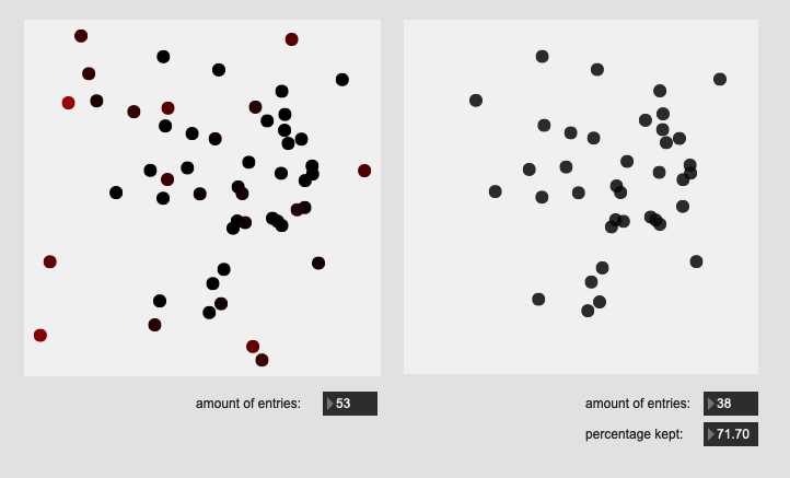
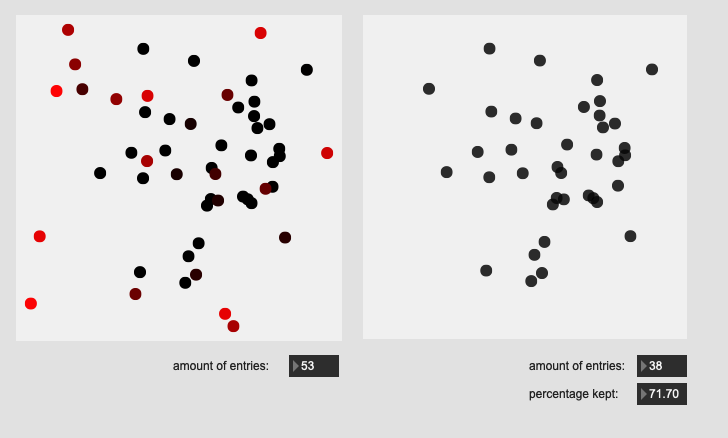
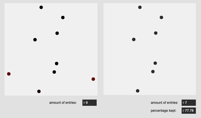
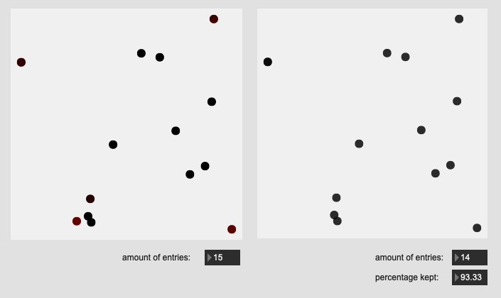
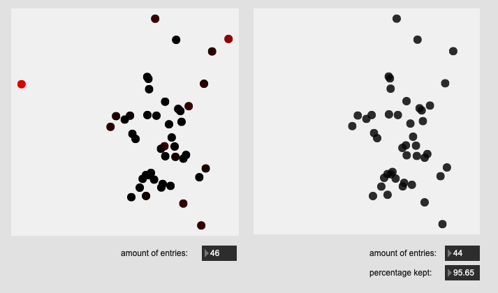
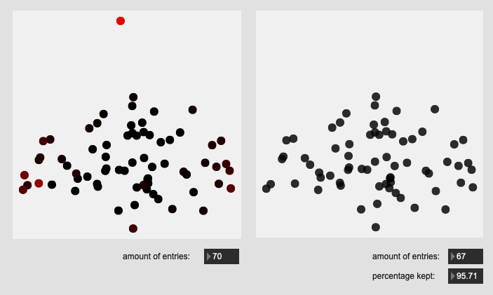
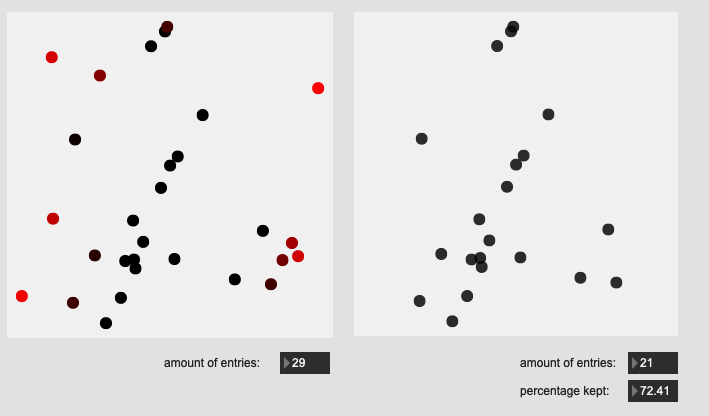
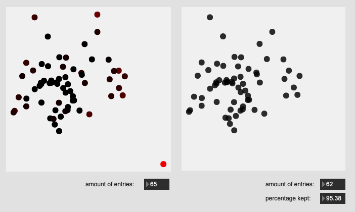
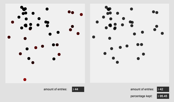
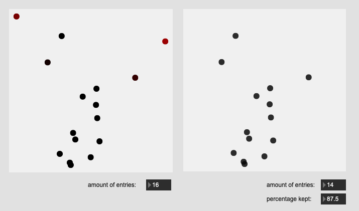
Here are some results on more real-world datasets where each class represents a bunch of actually similar sounds. The dataset above is one of these but with a single hit from a very different sounding class to act as an obvious outlier.

I’m really pleased with the (visual) results. I look forward to testing this across a few ongoing research strands.

Center hits on drum:

Edge hits on drum:

Stick shoulder hits on rim:

Stick tip hits on rim:

All of these are doing the outlier maths on the 104d space, then applying plotting and removing points from a PCA 2d projection.

I’ve yet to do testing to see how this effects classification accuracy, or the ability to “interpolate” between classes, but it looks like a reasonable amount of data to prune, and clustering still looks decent enough.

So a couple of follow up questions based on the patch/code.

//////////////////////////////////////////////////////////////////////////////////////////////////////////////

With regards to the numneighbours for the outlier probability computation. You say:

Size of neighbourhood for measuring local density. Has to be eye-balled really: there’s a sweet spot for every dataset. Too small, and you’ll see ‘outliers’ everywhere (because it finds lots of small neighbourhoods), too big and performance starts to degrade.

Is the only danger of “too big” being a computational hit? In looking at the code, it looks like this parameter just caps the amount of neighbors to search by, so if numneighbours > entries it does nothing. In my case I rarely go over 100 entries (per any given class) or a couple hundred in a really freak case, so would it be unreasonable just to have that value topped out at a couple hundred?

(I can imagine this mattering a lot more if you have tens of thousands of points you are trying to sort through)

//////////////////////////////////////////////////////////////////////////////////////////////////////////////

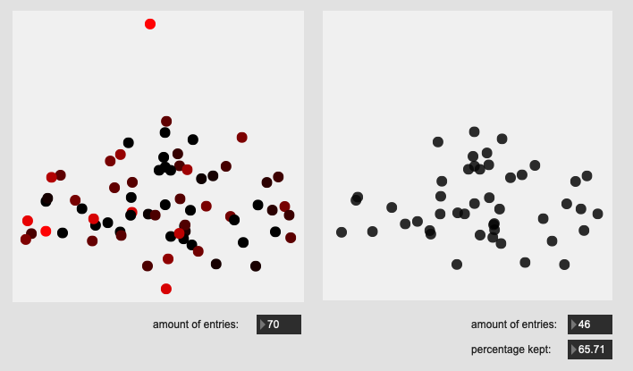
In playing with the tolerance, I’m unsure what the impact on the outliers as compared to the thresholding being applied at a fluid.datasetquery~ step.

As in, making the tolerance smaller gets more selective at the algorithm stage, with a similar thing happening at the query stage. Is there any benefit to messing with tolerance at all vs just being able to tweak the thresholding afterwards?

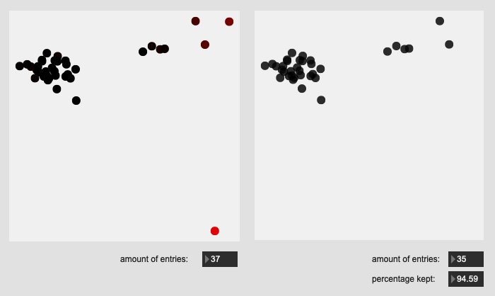
Here’s a comparison of the same data with different tolerance and < sttings, giving the same exact end results.

Here’s tolerance 1 + filter 0 < 0.4:

And here’s the same data with tolerance 3 + filter 0 < 0.15`:

If these are computationally the same, I’d be inclined to leave the tolerance as a fixed value, and use the more precise thresholding afforded by < to to the pruning after.

//////////////////////////////////////////////////////////////////////////////////////////////////////////////

So for the examples above, I’m applying the outlier maths to the full dimensionality, and then visualizing that in a 2d space.

Now I’m still experimenting with the accuracy of this in general, but I found I was getting slightly better classification results using PCA’d data to feed into the classifier. Similarly, I got better results for class “interpolation” on the dimensionally reduced data.

In a context where there will be data reduction happening, is it desirable (as in a “best practice”/“standard data science”) to apply this outlier rejection on “full resolution” higher-dimensional space, or the “actually being used in classification” lower-dimensional space.

I can smell an "it depends"™ a mile away here, but just wondering if there’s any established way of doing this and/or a meaningful reason to do it one way vs the other.

//////////////////////////////////////////////////////////////////////////////////////////////////////////////

Somewhat tangentially, a comment you made towards the bottom of the patch

Not implemented, but once fitted one could use this to test new incoming datapoints for outlier-ness in terms of the original filtted data

made me think of something like this potentially having implications when trying to “interpolate” between trained classes. I did a ton of testing in this other thread, but one of my original ideas was to compute the mean of each class, then use an individual points distance to that mean to indicate a kind of “position” or “overall distance”, but that ended up working very poorly.

Part of what seem to make this kind of outlier rejection work is that it’s computed across all the neighbours in a way that doesn’t get smeared/averaged like what I was getting with computing the distance of a bunch of MFCCs/stats to a synthetic mean.

If I were to take two classes worth of data and then figure out the outlier probabilities across all the points (or I guess doing it twice, once per pair?) would it be possible to compute a single value that represents how “outlier”-y a point is relative to one or the other class?

In short, is there a magic bullet to “interpolation” buried in this outlier probability stuff?

//////////////////////////////////////////////////////////////////////////////////////////////////////////////

Lastly, a fairly boring question.

Does something bad happen if you arbitrarily create gaps in a fluid.dataset~/fluid.labelset~? As in, if I use this outlier rejection stuff, and remove a bunch of entries, so I now have a dataset with non-contiguous indices, does that mess around with classification/regression/etc…

I wouldn’t think so, but then again I’ve never “poked holes” in a dataset that way.

//////////////////////////////////////////////////////////////////////////////////////////////////////////////

So the tldr of questions:

  1. Is there a reason to not just use numneighbours 500 all the time?
  2. Is there a benefit of adjusting both tolerance and fluid.datasetquery~ threshold independently?
  3. Should outlier rejection happen pre or post dimensionality reduction?
  4. Does an approach like this have any useful implications for computing class “interpolation”?
  5. Can anything bad happen in the fluid.verse with disjointed entries in a fluid.dataset~?

:partying_face:

Glad the code is broadly parse-able too.

Yes – I would think that for more complex clumpings of data it will matter more. Like if you’ve got a bunch of clear bunches and stuff scattered between them and only want to get rid of the scattered stuff, you’ll need to tune.

More broadly, yes there’s a CPU hit associated with more neighbours too, especially in higher dimensions, and (according the the graphs in the paper), accuracy steadily goes down once you’re past some sweet spot for the data in question (but not abruptly).

So, if you can live with the CPU cost and it still does what you need for a given job, don’t sweat it, otherwise use for finer-tuning.

  • Is there a benefit of adjusting both tolerance and fluid.datasetquery~ threshold independently?

They’re not completely equivalent because of the non-linearity in the way the final scaling works (clips at 0, meaning you have a class of points that are definitely inliers). However, for practical purposes you can probably usually leave at a value that gives intuitively sensible results for your purposes. As you show, when it’s lower, you get some points marked as possible outliers within the main bunch; sometimes that might be useful for surgical stuff – so, again, perhaps good to twiddle for fine(r)-tuning in difficult cases.

  • Should outlier rejection happen pre or post dimensionality reduction?

As a rule I’d say pre-, especially if the DR is just being used for visualisation and the actual classification will be done in higher dimensions. Nonlinear DR like UMAP, in particular, is quite liable to reduce the outlier-ness of points at some settings (which you showed above), because it’s trying to preserve the topology of whatever you give it. Because it also uses a kNN for part of its work, the two things could interact in surprising ways.

So, the it depends version: generally before, except when that doesn’t work

  • Does an approach like this have any useful implications for computing class “interpolation”?

Don’t know. Will need to remind myself of what you’re trying to do there and think more about it. But just have a play in the meantime and come back with Qs.

  • Can anything bad happen in the fluid.verse with disjointed entries in a fluid.dataset~?

Nope. They’re not actually disjointed (the order of entries isn’t coupled to the IDs).

1 Like

Cool, that makes sense.

I’ll experiment and plot more classes to see how it responds to this. Based on what you’ve said, and on the ones I’ve plotted, most of it should be relatively even/clumpy given that, by definition, they are meant to be examples of the same sound.

I have noticed that with some hits (e.g. rim tip), it does more of a sub-cluster-y thing, but still in an overall dense space.

Also sensible.

I’m mainly thinking of what parameters to expose for tweaking since it can be pretty overwhelming, and often somewhat dangerous, to expose a bunch of interconnected and obtuse parameters!

Right now I’m leaning towards exposing all of it in the code/reference, but only mentioning an overall toggle/enable and threshold parameter in a helpfile.

In my case the classification may happen on the DR data, but I think what you’ve said will likely hold true either way.

Was mainly thinking of where this should go in the data processing pipeline, and “near the start” is the answer.

Thankfully I already built a bunch of plumbing to take apart and reprocess data/label pairs from a larger dataset (what a pita!) , so can just slide this into that.

Indeed. That will likely be the first real-world stuff I test with as I suspect (hope) that it will have some meaningful impact there, just by making the “gradient” between what a class is and isn’t more defined. If/when I end up with some concrete questions, I’ll be sure to bump the appropriate thread!

Is that stuff in sp.tools or something? Would be useful to review, see all the stuff you’ve discovered you need and think about what could be folded into the main distro or a sibling utility package. Obviously we need iter equivalents for dataset and labelsets, maybe group equivalents as well. At least in Max/PD, ergonomic challenges in SC might demand something different.

If this outlier doodad proves useful in the medium term, it might become an external one day too.

1 Like

It’s in the sp.classcreate object in the p writeDictp info subpatch.

The summary outlined in the interpolation thread is this:

  • unpacked fluid.dataset~ / fluid.labelset~ to dicts
  • dict.unpack data: just to get the data bits
  • push_to_coll to move into coll-land
  • use the label coll to fork the MFCC coll into a separate coll per class
  • pull_from_coll back into dict-land and load into fluid.dataset~s (one per class)
  • tobuffer the fluid.dataset~s to get them into buffer~s
  • fluid.bufstats~ to get the means per column (now channels)
  • fluid.buf2list @axis 1 to get the mean of each class

The code itself is this:


----------begin_max5_patcher----------
7304.3oc6cs0iqiaj94d9UHz6qcT38KmmlryhMurA6CI.KVDDzPss5t0LxWV
eYNWBR9suEIkjkrojoror6YxzGb51VR1j0GqpXUEKV7u+cO73Kq9R91GS9Tx
eM4gG96e2COXuj4BOT89GdbQ1WlUls09XOtL+yqd4Ge7I2s1k+kc1KuI4eCM
qLOaS8cJlauN7r+NBs9hK2unXYY9N6WE5vEWseW8UwUWcc1tYuWr7sm2jOam
qChI7TzSIDLOkRobElp4TlRgvOkHz1aQRQI+spuA2W5tutN28we7wj+l4N+i
u66L+5ooifwx3PvLJ1PUXjHURwFRkJIHMQQ9nQv7XMBSnFxRvzoRFgiwBhTi
DJo9iFEGIdZAh4FhwXfh0NFZpDSk76.EOaUYogng+777rcYdHbsW5F6ktY8S
2DBJEwvh5ejXFPobbJ..TBuR3FoLPCO.T3oV+u4w1l8y4yeF50Py9b1tcaJd
Y+Nm5tGZ.lGdLewK4yaM5AcXniVrsX0RyUE1KZA3I.lKydIubqGfVFGflpjV
FLFIUSAkGTDwfuRkAZwzesAseqLYS9adfSpe7j3EOICw3xREs9ATS8TBSn.M
zJipJsDtDCQeBP9.A2XJAuNY1pEqgghev7j+o7rka8NAEZDnwPJrwjtngQLl
C5zzzZUYDrUJ1MU1vnw7hY6.NirMe8.ilsQy2bLi0qEk4+b9lZFIbM6U150s
t7Cs9HF76GWY+hTO0bohktKIZtzl7etg+j0b0rM.ouCn68ar81G+hf83gulU
yy2rbegsq3tHLRV0kriYKyVjucc1L2G1LzVe6VrVbhUTEKL+QQpl72n+qFN.
th2JWM6mNRnZ057kEKAQqs4K2ksqp22b644ulsub2yutZ4tsEey1Gvl1xy8e
spO58lFpvR.+gMEYkMjvaaJluZooSzYrvb45lCXUrpwwcHF6SrLasmOrS0RO
2bKPj629R1FyP0Kk4s3cAYgUqJ6dqlOWY9q6pt85hkKOBE2sZc+2bSwauOvm
8kUvMWLz2s8Naed+R2cAE+a28rQMZ2mKqrrRzt6W+WxVVrHaW9tB2P.A0by7
kY.g991YafIT5Put67ydtybfKeV9mKlu6caC0lY.d7h00LQO1LJOu3s7s65d
scYuss6U1t6qNPu0k1+RkT7y6xWrtDnhtO.HeTrc212W84sUOXMiVa.3feJs
kpaqmry0GRe4v14ch+KsutOy85WmYu5MEFDOQxSkJFAKAKc0BXVYul4NngeG
l.8g5oOtwvCdBfGZ2oUDD.XTRbJlyPLvrQf6GrVlcuPKXN1EflVuv0OrIGXv
SxR1BzTYdh0XuYfxyrBPG8aIf.dxe5+7G9gsIYKmm3L+y9xcumurd1ayaRV.
ydm75pMI4YydOY+xh+u8vWmoSj1tkKKVlOa09k1lm5eLR26XDt2wHzviQboy
3wpA.6aXRy3vMBnqfp4VbZaOLmx3S3N5Vy4oBMFQDJhD7dSnnV23rnA5FBCu
jALU6Vk7V9x7MFNugfCd7giJ+ynN+Xo5aN.TBycjr50NBH48A.z3C.To9TkU
UvAdZfiAzVuK4kDPeyP5qE3K.DnmADXBOZrsSxgIrvzQa3jq8zzQ.2NcI9TZ
+4hcu2VAsIhHFEzuTXrtqOMvj9PczDH6IndX8PpTkliA6ILtipvRlwta6XAk
dK4Dmuew5gYE4WBqHID8y9LsRxCiQzzumHlvAvqebUwxjueG3nwafGrI39vL
lnWLiboFbQOR5kKAoWvkcphy4DEQyQbfKRS+fYaJ3xK3a37js465Ettj47tD
3xm4oRxGL.yDhkdQJ1EvXwGORAVMkpIDNkCXDGokHhInQo7fjMODinm5I3jg
Dfxtvmm.UVEuf2xl80iXHLz4Fv+zcf+rNGrO4yc3AVjsdcyiz7DMiwStJ3xj
xdGtowW2KUqSwGOgDFLUlRvfPAVJzBshXFoYpvFvaEhzoGvdsbew7zW1+JwZ
U42m8khAzDS0wWSLFDNNQhQpwoBrDIvLPZAQoHwAiKOKBZHkGuo1e1KfIiOK
mW.S.JdoXLWYVSMClQ.uy37QZG5MeVrU62LKuWviD+IxvLO5mklXCqfovTfI
.ZsFiMJs+nMS12JS1VVLKuewSxkXnzEwsQIobFEoEftOC+FQEN21MkSayJav
kVAZ3dMuWqxI7aDvwAtJojIPLEkYfMJq1qwOpSLXV5gs+yjueadIPa1fszGL
hk2HXD7wIUwTbIBK.CpvDL9Iquge7vwcMLeNuCKSPC6gH9RrRgeIVonAAVEX
dB3prlIwZr1D4FhIWiN7iDGBjdP.6fyjl+WXB+vs1uRPQYAXJZ+5Iwn3ym5G
hw7TvcRIRoXLlPZM7mI+Pxl9xP1wfzwOBZdkrofG2Zv1YlBCbjJByvThUjwY
HyM2fF2zLCOICZBljgH8DOLFbQFHVSQJJ37gPXxGA4G2IYLlqS.rqWfiEe6.
8CbTZJ3sgfp4HFSw33QDQipA+aEzYC+5.La8OKBuWLicFAVv3E7wBr9wLTpt
8ORRHHX0jEsm63l4PR1reJIa970qfVMo3bRx8GDWZTcCliooDpTPHXgloTR9
XzFdiEiMqVv17c+S6pmCepmGxTQD4F4XLmCVEhDfYUfchZMxt1.R1GUWU5aU
c02HKqobFHiSEbghBbbHpIzUJ0ox8ev.Oy5W0C1ItjoOXWB1gYozVqCkMDLn
QDzuoKttdRB0aYXYclGs8qKdYUuiRzIv5HL4TaxITVphq.snJv3RICgggI4G
QaxecypEChYb8DDfLeb1dcUTh+nk2VmmKiqtQ5Q8tD.eH4xrqBKs05vR5C6X
2HqdHvzyBhISygIpYRAlJLnF9Rro7lNAj2s3vIvHJ9SG4UQmWgVO6.h+UbBo
d12OGOVwzwerxksFdiLjIKP+WkAGKR1aBawieJ11N6Mon5eGP7j57H04TUfI
h3x44eo0dj3Ffbp3ibdS0swAj8ChAjLi0fHIhfnqG1KJNAoOr2DCAbOncN0J
0xdwz1f1.YB7PbbG1GJlD3qmcWfsqatueTrZIacCq0tllzsqNOe6thkMaKm+
ZqfHmDZ13M1tgwKuf5FxIsWPCrWXLlJAOQ8BtdL8hoBKL1ZGVu3zt6pMycaA
N7ctqgN4AWT3hR315cvM5zfifU7TIhyXbEiRHHkyXU7opQ87j9ABzz.DgJ0H
lTNETn8B5D1KLF6YDIOOSgZp6EAK6RFh0TQLwdByjo7icCfRndbX3zmbhHRR
fznGv3XwOg1RjHAPOJlfhkJBPYL7S0z+o2ZhnJqwWgMUnYGILYrPVymCqevm
19ANz9AictAZJWbJGqFgS0BLA7ehIIblhiM6M8SUH64AmThlLFhdB6GgnNyl
NDSW+fGZ+XRmhogSOXcNSS2vrWFBTjfOo8C9XEMmn9AKXUlS63BMToEOifGo
pRPUmppRQHoJNkJEbDL6qjy5QUkmGbRI5f.e7TZ3kMsxCjYTLgtMYyV6vXBn
jIEOjAOtHmz9AYr8iALTi6gWWxHoLA33CiYVgDDFYbdxmGUddxohpIAqhlNo
nOIXUz083ooefClajNopns5fHgFgG7PLibDpaVtZRZIJimhOdYmvJcPO4jRz
iw5o9IZFmY7Ghh3oDF7OEGAy0.+R2iLmmmbRISZPAQjdN2d4LOdJv.GdUGka
FDhzSN.dxCNozbXANkb1wVj5TRgynoblTifgNtodJZhBk2QZOO4jR0r3P0b2
dz4iIchB1llI01JaP2CxcTDax6G3fkvm19QXRcSZrQP7Q0OlL9TTvNfglTGR
QzQgGSlO.nfs4kLs3AdryNLM8i3EAOSE4zaD73TEQAV0C10q3ZU+Qv6nGzKI
Wcw5pQXn0syQUD3dqb0KYkGU417Ui3hd09zsMcd4jRdSmJ9iZDERUw.EiYbJ
RczNAyakYFqkoZdqGkQOWgu73MpyIabmi1zXwC8JGB4DQpV+x6uLVi4ATcea
CCWITrHe61r2xOstote66Oua0y8WZd8Uje5jHaz3TRUqQKeErWs8VTd7KHzi
AWZWYnOKpPhTglkoRYsEprhe9vHEapvndDiZURU5jrbpQP47yxO3sp2eZ5ze
QELkKuZNeZARYvhixfEFkXNwPeiIx3LlfAlLvmoC+XyS2eaDZjiPo6WZ2oYF
EJexyv0Xl+gLtYtkv3BEIPLg6PFPJ.sq5fKX2iaTo0XvkiicKecG.RnKtduM
mAq1wYgpZFOBzE0O5JEo7iQWhLkgv0SzSs6oDttaAnajje6z7zWAc7ZOpM7v
iPTo5iohSyFwAxtyNIoXuiScyQwHwUrc2pMl5YXc9jBMRwr7sl7ycQ1OkmrM
aw5x7j0kYe8EiH31By623k2g5g2QDGlGpwlPtQzC3NPU3LLWNybQ7wEU1HgM
lpgPlsF6tY092d2hQAKzvhCgyb4esuRkua2XdwBJ8Q0VpJIag8OGxv3wYjKl
DGxG7RGbRpkWsbL23nqY+8dzwnfVMIvwl7Eq947j46WWVLyvMLRfHRZO0Zwo
3.UiRA1gJqZA6ILkEGWvciNNbfg.t6lhbuGWDnHMpS01i1.yhJzVZmSIdpcx
Qh.+KF0clxo8AEvl2ksLq7qeKeds13VUiafPruqpnvVr7UPoY9tLa8ec26Y6
R9bA3MzKfVTiV14tBEq4K8G2tZYZn5PUQBTIb2V4fe5rUD2zUwWCpARLVvUA
p9L0NNTmxsAsTXcJlgH0pF3TSA2bR3WNvlTyMDpNgHoaj3RTSeimWoMT8XJd
4pr4F++SP9N71FCa5fmTLbqruDruFynG12hRuUikI1mcSnuv9nVYbb4.iIV0
0BELJ15.shZpLbmts15OjWGp5Gw6LMaQ45caxZUDq6f.w5nbqFA7cTtou0Gr
Yg3sIgEmw9p.17KOOLGJH6dwqXIrfvcy7.qQPboLkxvM1.YVIDgJbImpMq3s
.GhTbJ.QCqOAdH7PTPNYD95DygNzeX47+irlJxRW.fFm4HjJZuSQnCaJh+06
TCiVUQtPVlGkyMAlT9aGZX+1gF1ucngccGZXAcNOY8Cx377WO3H3b6sLGpS.
xa7kv5tIzgSG84FxDbj8HTtyvRkrZ4KHL2Jl8TRkU5Q+bBYHjzfQ+dKh0BnR
L1pA9VmssBhGMvMAG0OUgu.Is6jN2Az3MEppqwB1ZmauLYiEplfs2eSPL4tb
O71e1yXivqQuW7NXvHmsjFXSIZRigK1ZEm8jbNvRczbqEVNQhaWwtc0fEIJ1
DTVspBjgIdu75vZ7Ap5E0DQjeeeXhXBpAqLWYXThS8e3eemAEWkwpO.gG+pg
UESB1pskp9ngG6WNHhbQGWCmoXIwbkYFrBYkaXX8EUNE+PfOjInXR4SCbMXw
urJ80M5XYJq2ZcJQMAmVe9vIpc+vnPL68jrJaCY5fOiYd5veukUq3pijujul
msI42kr.747c3uyy9Z6x3Wx2uNa9byIvJIA49eeHN6BJVzjPzkQHUVW+Qr5i
WCiuuZ+F38.UapejeJYKX+HXjYvvGVGe3iQZieDk3dgeCUswjrInXi4QR04o
VbKZag6PwjTD2Fr9iImfCwWm7HCMTYaqMNMdeTuCkdrfq4Wm7byVU5hn4e0F
UmV+BmNU6khP2GsD0Y6t3aT2EGmtKJ0T70E3pNNNcvMJhllZxLMLsNYSMkrc
SHxsl.xc2ryL4taduqHSxAYyv2J1rfKwH1Z.B9tKVDboHwy.w8.eCupHnuHA
ioqSiCsSS9.0oIg1oYeL5zjPUWPXmEoORM+P6s+S0JRvpTg8jGs57H289ojr
wgR1r3P1bociBxDMowrgLQNx1bL0yad+TR1jPI66+j51IqCYXxiVt6mHUn0U
Oh9iAHyFyLv2+9KVOl9aTlb3f+.1kBsGGBNrR56mWr5OaWO6m+S4K2evui5U
d2Oo9xauVTV1zGe3jm3gGA+AqVZb4g020cm86V81lr4EU9D04lcnahlgwJCw
aqoDB6qfWv4GIrU84v0ePFmoMU9c3UBhjwsuRQnlz87Huyp9njCsoAmssDRq
L1HadUCz28itdyp0q1zjxCoTc66V67bEQ4sfu+TKtqM.fb5JXaTOCCDEsqVs
93NaFT+u1OKKzAxrYyfFsCnSIbSn5fWXNS0cnuzcsim13k257I0HFVZ+nJMm
Ik1WwHZoE+4hi9r2HVnQLb1kIR0v5njHtR4dkhQ68i1vDIpQNaZnIcux8sco
7PMjaK1n9zWvjbL01yIZJLVXeEGiDdFCyKyWbLKfTAcZGkivJk6U.2.gb5mu
cl4.py9uWmuL4OmsbaxeNeQwKqJmezAof83tEH1tMHA5aV.CKjDmPpBgLEEp
iaOSXFse1mKVZx0p7lQZplfENRsV5mzd3ZRE59oskEyy27+XRSqPE9N1KqN+
Zh6ut329uWtO+2guFkEXof43ua.cs4R3aHQrY0mWdUTwg9NW1n86FSE+vWyt
Nh.Q.ktV9eojRINsuDL1ju+2Jh3OtIO+JoB6nPkOGF0AFsv2NB3+Murb0muJ
JPAZZsfuTgUXqpLNLxv8q5rUJJRLOHBolZBc+hWx27GAMyWEYZDOPV1MNn2k
aoXb6IVmThXiScqgJB2l0w0+6axUvsXAUWIcIqrxAFe0wSN6W2EaG6dnndGT
j+b8Fn6SI.m4yUadP2apN0Z9j63q4YaVL24wddc9F2SU+LU6O452ZOHW9Txh
x0OWsUU9Tv6BKl+cqn9RyFctBLolIYLrxraNH1svilAtnb3Gl7bkbjVE4g3t
oDJ8uoDnQZSI.xJtcnMhlhAmCZ1g1FcjBZX6mknukD5dbO2kv8uAl3itpEIb
4gklpgweU813QoMFlJvmmv687aNZklmxxmMGJl0Emmm6HJEr7BMREtHvOEwo
aiGA1TiIw1sysU.hb3X269WjdHTVjpHLd2CSd29e+VIgomwHS5h4cLJR0PpF
UYRNvRpa184XS3kBRUVbUgMfPaGxGGmxvlvc1v.BimrUpwTdfaLw3wE54TUL
lLSvW+57kycaQeevZS9GdkaZsZtJPC.LgASWWLOvBiqopOtrUnHUc+Znelot
GVW5NvJDm7qRNqZD1rsj7xXohj7Jh0WIhInMC4uHA0SbPvKBKipFQlPkJOtr
y.tV9KVLNbKF6EtOqUiDQblTV6R9N+lIREePLSjDIyDqo1eytvQWkeK8WdRH
z3nKndy26y5nPFY7Uxdicw6Xmsb8B+yKPPhDPvrJ9.tSSAlto7Un41zNb7JE
iG4+MfxyWl78eqDdZS.XSnDXHxKXfFg75PklBJ2U1szl7v9nJxElgCtbdDUT
X6pM6BBFvr3.CT1Pn.+NfB05D9VosXPmz92dKrOipFlIOKTbr3ghY1NVjQVk
NpjRpHhCk151uH1JQNqiQnH4XDyseFOwuHpwagateQ8EbAjJN1wTQsGEaA3U
bW3t32TpETRrI+MuzqLNpDpmuzi2Ib8cQgPuyLhFSnvomWKn.kBVlxOTnmMZ
AQD8HlZ7NMsHhFoAem3qeGmtWyJtC5jggB7HgBNKk9PMqX+BA33HDTGtGkP.
tvzDrGtMGsvX4cRH3nZXPWRGE2H8o.m3jLQS84hZLMNnvELEA5KjHlf0533b
Pyb5ci0mTYml6WvgLoe0JlpEsWSJwZUbziTyWI0Lv1Ady4ihFwc0t0atdjyY
iHVRhiHEXBcZeJSt4lHtqYKM2sTmKiCsBSQj5YTVXREEBIr0SNlj6alcyJwO
qsPDIGGqnYe4PAmbG3rskjhCUE.+DOKNtDTyb6a5BM8dTwa8lpHXtNNlFHPh
dq3qbw3p4sSQRiT3k3ik+e.wy6o1Uh02Aw6s4kIH+L3b+R2zwNfycaoLuwtW
dIwB41jhPXdjRQnZ52Wz7wH8sKEgtrUpDyYwwpvJEcGmhXDqhNzuBsIb16.G
qOCihjmkU.p2RfL593csyL3P7uFGIyhqOhT7thLj6TLmK85HPbR0xp3K48bD
CinguFTwdr+sMq1uNrPqD20afPS0s.BJA2TgRuCq5RYwr7dVbgHwwSr1PPTf
+fzVYRiY+TwuGwSxlx2E8jnsQxEvZhlaNPaaMKpIRxrIKnJ8cbh0SVggtvSw
SeGDZw3HD63iljlhMD4BvhNEeoNkvvXcDwopNDWXmnI2CXzlh68flw2Yll8a
naAUxQ9GuAvq.gS132cpTL8UH.TGNdoOAmCsg3z.ZIVTZIRHsjLFsT.Mj005
nzR3y0RbQDZI6fM+LMkNVMD8LMDmDqVhcKXHnp.FmncJRTGWPSThTpr04rp4
jzlIL6Y3ilcjPYcNizkLh2mLFjz4XxsGGF8SSljI5jSiTrYUTO3.M2j5vRs8
bfxy8hAUPNm.jDECd.YHZErME9ZaJQ.hPQguNjoIp0ve8sD9VLMgskNKKQTz
zE.3ECU2cq8MmoJDccsTXJEL73x9TJfwBtKP4lXEyZNZDQ1UT2dRCzRkA0bU
OO50RHxqW6FFSw0Zs3Lpn1XOtwXuVZzN5dwnmiCcH35ZpPrygDC8LDVPiGTV
zZqyhfTZTZqPTqYSv7H0VmEC6VgpNwJDkMZbBIBbegzDLBgacbz8buqtmSCV
sx0iRnP77AGklJjVJJC8AM6oc6BGo157hpjnzV7faK7U2VrfYB4WcaQucp6n
jfTKniRaEPSoGbNUWk4GzH.NBbHWKQba.g0l0d6fiOVugN8IuVhHLyonQQaD
YT5rux1JbFbVeiOUyA.9blJN4XKzb5SzxxMB0+Sd0zAMHKfFzaaMkj11JSqq
obgY07Q06BDjzVD+LGe63SNwNO8QiBYc9gmnLegssnAMewAOkduX97pyYvHz
5m2Crt9ZDuVmD.sS6Zi3wbOBlayThSwTUUh9.rBlr+vbDk6I7Lm7jW8PHIXo
YZuV6wcIxAxrn9MFzIQZrwZOZZSME17C2+SFE53bLC1T4OINs0Y0bfhhk+DT
viO3IfIOjFOJF4hCZVEbTlsDiBIzwQqk3mUAItCsuZyb24vKJBMN6rFEntcD
5QgKogPwQnwQAI626L4TtMHLLsDL9n09yP7Tsyrmdqn.ZmcBr3M9HN6ZMIFB
h.RtNfasTdCfgoRdUW4uN4dQome90tJNnTP50GBiXtj3ihMavEdcx6xTXxS0
rXdt201uQg3pgcGMb8XDJnX2hhSaET37HQYhVTHwyuY53HzVmexNVzZqyyTG
ko6PAEmERThoCJ7f8MA9dfvA4beT7xBElZI0P5kHRg8HcToMNbppqiWbpvdh
HYyTNO2KJc8yNCGevXICckpttImok0AnQwklb7hor4Iyo26p65gYTQTL9Mrl
JFLSG6NbesEJJsUPKZQrZITfSbecsTHvWLzkZ2uXmeNcNKJsU3NYJhttTbHS
xOns6LlsZyXJbZTJtIY54l.GZ1pw9u20BZhfRTigMotxrYkIgNasA2LkPapK
s0G3VFisauEw5XEd6ab0TpHHJMFqfqqsvAkTb8FWMF1luyJDOE0B5jl3QIb6
aPO26p64rfRbmnnuiqCZd0AMIPvIt0gUkxNdq3TgfdtWT54mWsFOZnDNn1hb
0skJXsAWMmFOHYDtNJXn3FNdETBwxUQACCJdin3zViYUZ6YAMIzFoUJibH63
Qr9VaIOOZrCwXXTF4xorlbEI.R4JsBgNlUqsGMpthVDz6f4e4nZ8lLEwte0k
V2X7c26BwzDOnwQLhF+EO8VCye41rAYqWaNLip5KVR3wEY+n6TmP8j8sEKcu
UXe6l7etYuIZ2RkOlsYl4zGZ1t8abGlCeoZCn+3hUPCubeQEFZOWIdztuMrG
oBqyb3jc6c7c+iu6+G.0IE5M
-----------end_max5_patcher-----------

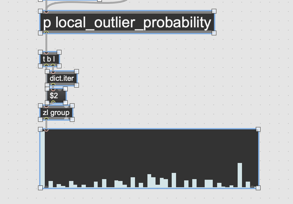
I’m certain there’s more efficient ways to do that by not going into coll for the heavy lifting and just doing whatever is needed in dicts, but for me the most confusing/challenging bit was breaking up a fluid.dataset~ into separate chunks based on a fluid.labelset~.

It’s kind of a data uncanny valley/blindspot in the fluid.verse where the fluid.dataset~ is a monolithic thing, but when working with classes (or lots of other use cases), there are subsections of it that carry significance and would be handy to break apart.

Hell, just being able to use a labelset in the context of fluid.datasetquery~ would help a ton, even with hose tricky to parse that object/syntax is. Beats dumping/iterating endlessly!

Absolutely! Could fit into the ecosystem quite nicely.

I took a crack at this. It’s in a subpatcher here. It pulls out all the IDs of each class and collects them into a zl group. Then enables iterating over the IDs and playing them back to hear each cluster. There’s also a subpatcher that additional sorts by distance from the cluster’s mean.

1 Like

Ah nice, will have a more in-depth look, but it looks like in this case you had a known/finite amount of clusters, so could make somewhere to receive them all.

In my case I wanted it to be more generalizable to deal with an arbitrary amount of classes, so everything had to be iterative/dump-in-place kind of stuff.

I remember running into a similar issue ages ago for merging datasets (also quite faffy), and @weefuzzy came up with an abstraction I still use in a bunch of places (I never remember what I called it!) that just juggles the merging (A+B → C, etc…).

It’s a shame that stuff like fluid.dataset~ didn’t happen earlier in the process to have some of the iteration/breaking-in that other stuff did, as other than having fluid.datasetquery~ (and even with that), it’s really hard to do anything with the data once it’s put in there.

1 Like

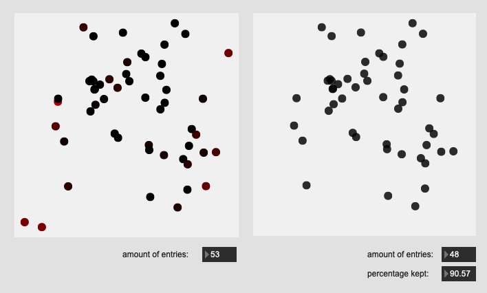
Ok I ran a bunch of varied class trainings I had on hand just to see if anything didn’t work within this context.

Some slightly surprising results.

Firstly, a beat boxing corpus, which has quite a lot of variety within each hit (much more so than the snare hits). The amount of hits per class is also quite a bit smaller.

Beatbox Kick:

Beatbox Snare:

Beatbox Hat:

Honestly, I was expecting this to have much bigger outliers given how it sounds (this is the beatbox audio example in sp.classcreate).

Then I ran a much longer/bigger/comprehensive and slightly more varied/casual set of snare hits.

The snare edge was very similar to the one above:

Though I apparently have a nice big outlier in the snare center hits:

If I run it again with very different settings (numneighbours 10 and tolerance 1) I get this spotty plot:

So I guess even though it looks fairly clustery, there’s a good amount of distance within those clusters.

I was quite surprised with the next two (rimshot center and rimshot edge) as they are intrinsically very difficult to get exalty the same.

Rimshot Center:

Rimshot Edge:

That being said, the overall spread/distribution is bigger here, so I suppose that’s where that variance is accounted for.

If I try different settings (numneighbours 25 and tolerance 1) I get something like this for Rimshot Center:

I’ve yet to do any qualitative testing with this, so not sure how this impacts the accuracy/matching at all as I’ve just been staring at plots and massaging numbers. I’m curious with sounds like this that have a lot of natural variance if it’s better to prune it down aggressively or little at all. I’d believe either.

A couple other classes of note.

The Crossstick:

I was trying to get a bit of variety here as you don’t always line up the stick in the same spot, which I suppose is represented in the little cluster islands, but one of them is right out there!

And here are some more normie ones.

Damped Strikes:

Shell:

Both of these appear to be a pretty even distribution with a good amount of variance, with the outlier pruning just nipping a bit off the top.

/////////////////////////////////////////////////////////////////////////////////////////////////////////////////////

So my overall takeaway here is that maxing out numneighbours seems to work out already for the most part here. At least across the types of material I’m testing here.

I will check it on some other sound sources (actually quite curious how the cymbal stuff behaves as that’s a quite different contour than all these “hits”) and then do some actual accuracy testing with things like the beatboxing and rimshot hits where the “class” is actually quite varied in how it can sound. So curious to see if keeping an overall tighter cluster works for the training, or if it’s better to have a larger, perhaps sloppier, representation.

I see some of this inquiry leading back towards ideas of regularisation and perhaps quick/dirty data augmentation to perhaps address any funny business, but one rabbit hole at a time!

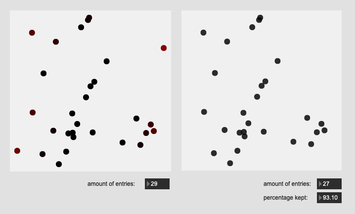
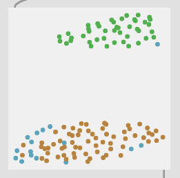
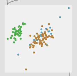
Couldn’t help myself. Here are some cymbal classes.

(it’s worth mentioning that I’m still struggling to differentiate three classes from cymbal audio. I can get any combination of two of classes playing nice, but combining all three gets shitty accuracy)

Cymbal Bow (middle of ride):

Cymbal Bell:

Cymbal Edge (crash sound):

As a reference, here is all three classes above plotted on the same plot via UMAP:
Screenshot 2024-08-01 at 10.27.24 PM

And again with a PCA projection instead:
Screenshot 2024-08-01 at 10.30.19 PM

brown = bow
green = bell
blue = edge

This is actually the first time I plot this with PCA. I guess I need to differentiate bow/edge hits more as they are all smeared in both projections.

Cool, thanks for all that work! My impression is that it’s working pretty well by and large.

For the cymbal bow / edge, I suspect you need to revisit the features if they’re that confounded. What if you add pitch confidence?

1 Like

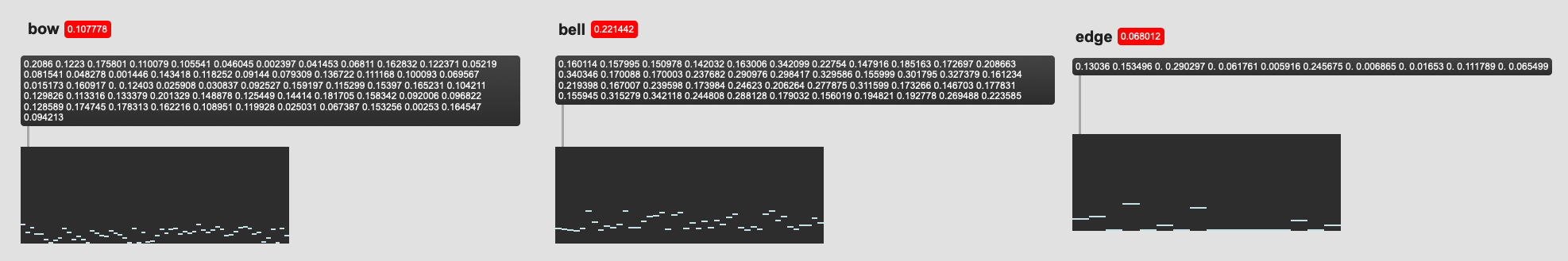
It’s not as straight forward to swap out al the plumbing, but just looking at the pitch confidence for each of the same hits (as well as the mean), and there’s definitely a bigger difference there:

Image is kind of small so the relevant deets are:
Bow mean: 0.107778
Bell mean: 0.221442
Edge mean: 0.068012

From the look of the distribution I likely wouldn’t trust that single dimension to carry the weight of it, but it does look like it does capture that variance.

But what is a lowly single descriptor to do in the face of 104d of MFCCs/stats? I would imagine that a classifier trained on 105d is unlikely to behave very differently, particularly given that pitch confidence is 0. to 1.

I guess I can try and come up with a separate recipe differentiate these hits more precisely. MFCCs does seem to capture the difference between bell and bow quite well (as well as seeming to work across most other sounds I’ve tested it on).