Class "interpolation" (distance to classes)

this could mean the data is all over the place for that class.

Imagine, class A has training centroids of C5, C#5, D5 - the centroid would be C#5
class B has training centroids of C1, G1, D2 - the centroid would be G1

if you test class A the distances would always be small because your standard deviation is small
if you test class B the distance would be all over because you have a higher standard deviation. but it would always be nearer that centroid to the other.

it is a blunt example, but I’m trying to pass on some intuitions on statistics here. higher dimensions is the same but much harder to visualise.

Ok I managed to plot the means onto the same space (basically inserted them as additional points in the set of hits, and gave them new/fake labels, so they would get different colors in fluid.plotter) and that gives me this:

Red/Yellow are the classes, and Blue/Green are the means of their respective classes.

Barring a few strays from red in the yellow, this looks like what I would expect, with the calculated means being in the middle of the cluster of data. I guess the blue could be a bit more bottom/left, but this is a UMAP projection either way.

With that being the case, I don’t understand how the knearestdist would always have the second value bigger than the first. Especially if I’m feeding in the same data as the training points themselves. Surely some will be much close to their respective means than the other.

Like when this strike hits:

I would expect the distance to be small for one point (green) and large for the other (blue). And conversely when this hit happens:

I would expect the opposite results.

As you can see from the vid above (reposting it here), that balance/shift never happens:

I see, the first number is the distance to the matched point, and that changes as you near the other one.

Queyring for knearest and then knearestdist I can use that to either reverse the list or not, and that gives me something that has each class in a separate slider.

This behaves more like what I would expect:

So now you can see it kind of “crossfade” one down and the other up. It’s kind of clunky and not super linear or anything.

If I wanted to have this be converted from two values fading down/up to a single value moving from 0. to 1. (or whatever), what do I do with those numbers? Summing and dividing is no good as that breaks down at in-between values.

1 Like

that’s it! Now I understand how that can be annoying if you want to know always 2 values in the right order…

That said, looking at your example, I think your training set is not so good - you should get a lot more difference if you have the right amount of dimensions… maybe we should look at that together in a session.

as for converting, I would probably scale and cap the distance to a ratio of the distance between the 2 centroids. this is a hunch though. another idea would be to make a ratio of first to (sum of first and second) to know how relatively you are far from each centre (a sort of confidence)

Yeah, that took me a bit to figure out. I guess it makes sense since more-often-than-not you want the distance to the knearest, but in this case I wanted a static ordering. In this case it’s easy enough to zl rev it, but I can see this getting much stickier if you want a > @numneighbors 2 version as I guess you’d need a matrix and some plumbing to reorder the knearestdist list based on the knearest list.

For this vid I just used the setup as I had, with data I had pre-analyzed. The tuning is ~20Hz diff (~430 to ~450) so not insignificant. Also using a different physical sensor in a different physical position (3 o’clock in the vid, vs 12 o’clock in the training). But yes, I agree, not great differentiation in that vid.

This is something I tested extensively back in the day (a ton in this thread, more recent optimization here for optimizing for an mlp regressor.

At the moment I’m using:

13 mfccs / startcoeff 1
zero padding (256 64 512)
min 200 / max 12000
mean std low high (1 deriv)

Which when comparing between center and edge training data gave me 96.9% accuracy. This was with the original Sensory Percussion hardware, which I’m now testing with a DIY version (much quieter, better dynamic range, wider freq response, etc…). It would be worthwhile revisiting the optimization with that new sensor.

(listen to the diff in these two clips, recorded at the same time with the official hardware first, then my DIY one second)
Sensor_Comparison.mp3.zip (708.5 KB)

Yeah, would love an old-fashioned geek out sesh if you’re down. I’ll be in the UK in a couple weeks and was planning on taking a trip to Hudds for one of the days, so maybe something then?

I was having a bit of a brain fart with this. I guess this is what I had in mind:

I had to do something similar with an update to my DIY fader thing last year and had forgotten what I had.

This sounds better though, and hopefully more robust.

Also want to try and streamline this so I can do more robust testing/comparison (the reason why I’m comparing a slightly differently tuned snare/sensor is because this was a PITA to compute).

What would be a good workflow for computing the means for each class in a classifier? As in, I have a fluid.dataset~ and fluid.labelset~ pair with an arbitrary amount of classes/labels (in my case, realistically no more than 16).

I can do the process above, but it’s a bit tedious and requires forking the process down into separate/individual fluid.dataset~s and respective buffer~s, which is problematic if the amount of classes is arbitrary. Granted, I can pre-bake a cap where it can compute up to 16 or something like that, but that seems needlessly fragile. (I guess it could dump/loop into a single fluid.dataset~/buffer~ combo, but still, tedious.)

I thought about using fluid.datasetquery~ to avoid going into dict/coll-land at all, but can’t process anything on symbols/labels.

I can try and optimize the above a bit to skip out on the intermediary coll step(s), but that only really saves a couple steps in the middle. Most of the plumbing remains unaffected.

Any thoughts/suggestions/shortcuts?

I’m curious how only mean and stddev without derivative would do…

why don’t you use tobuffer from the first dataset? your classes could be in 2 datasets to start with so that is way simpler no?

I need to set up a new/robust way of testing/comparing stuff. The patches I’ve used for this in the past are super hacky/messy.

The first dataset is a mishmash of all the classes. As in, there are 100+ entries, and around 50 entries per class. So if I tobuffer the initial dataset, I’d just end up with a mean across all the entries and not per specific class.

fluid.dataset~: DataSet data: 
rows: 140 cols: 104
0     33.909   -5.1534    7.4311       ...    2.0758     9.974    2.5649
1     49.644   -9.4954   -1.0355       ...    6.8681    9.5761    2.3219
10     43.111   -9.2246    6.9809       ...    6.0569    3.4346    7.2621
       ...
97      42.06  0.071087   0.74264       ...    4.9557    6.7441    3.3876
98     68.636   -6.1345   -5.1666       ...    3.4278    4.2649    3.4061
99     58.526   -2.4483   -7.2108       ...    4.1994    7.9537    7.1264
fluid.labelset~: LabelSet labels: 
rows: 140 cols: 1
0     center
1     center
10     center
       ...
97       edge
98       edge
99       edge

datasets.zip (133.2 KB)

ok let me think of a way to split by class because there must be a way - in fact we do that in pd as a “tobuffer” method I think. but it is too late for my brains so tomorrow.

1 Like

it seems your first x points are of one class, and the last x are of the other. if that is the case that is super simple, you tobuffer it, then use startchan numchans to do 2 passes of bufstats. voilà!

In this case, yes. But that may not always be the case. It will often be many more than 2 classes in a set, so my plan is to pre-compute all the means and then when trying to do this interpolation thing, take out the two relevant means and stuff then in a kdtree.

So is there a way to do what you’re suggesting 1) programmatically (without manually checking where the classes changeover) and 2) work with non-adjacent entries?

the simplest: make a dataset per class as you enter them.

otherwise, you’ll have to do it in max as you did - you could probably use the label dump as iterator to the dataset dump all in dicts but that is still you playing across boundaries. one day, maybe, there will be a sort of datasetstats object maybe. did I say maybe? the interface would give you more reasons to moan anyway :slight_smile:

I have a hunch that getids might help us here… this is when I miss @weefuzzy the most - his programmatic brains know no equals. I have admin to do but I’ll let that stew in the background and might come up with something.

I could do that in parallel (as I’d still need an entire one for the actual classifier stage) but it still gets problematic to do it with an arbitrary amount of classes. Again, can make x amount of datasets to dump into, but that’s kind of hacky/fragile.

Could do it with fluid.datasetquery~ if it could take labelsets as input (as well as non-numerical filters) (e.g. filter 0 == edge, then do whatever the syntax to filter one dataset with another is).

Having a whole other data processing structure would be a pita (though useful), so just being able to move the data around to use the fluid.bufstats~ stuff that already exists.

not really - you can do that in series. I reckon you will record one class at a time. so save in a dataset and labelset called input - that you clear before but do not reset the item counter. then when the class is finished, do the stats there and then and copy/append to the overall dataset/labelset. that way, minimal pain in training, quick redoing, quick update, quick addition.

I won’t always do it in order. Rather, the process should be robust to not doing it in order so you can add/amend points to a class at any point. The datasets/labelsets don’t care what order things are in. It’s just not (easily) possible to poke at a dataset based on the labels with the exposed interface.

For elsewhere in my patch I’ve compiled a bunch of metadata (amount of classes, amount of entries per class, list of unique class names, etc…) so with that I just brute forced computing means from the info from that. Still quite clunky, but for my specific use case it’s sorted.

Having a generalized example/snippet would be useful as this seems like something that’s useful in a lot of cases.

1 Like

I’ve been doing some more experimenting with this recently and getting ok results by taking the 104d MFCC (13 MFCCs + min/mean/std/max + 1deriv) and running it into a PCA based on some @weefuzzy code from this old thread. The idea being that you can specify an amount of variance to retain and it would then give you the amount of PCA dimensions to keep.

Perhaps counterintuitively I got better results the smaller amount of dimensions I kept, with around 3/4 PCs seeming to work the best.

After that I’m doing knearest and knearestdist (as above in this thread) to work out the distance to a fluid.kdtree~ with the means of the classes (also run through the PCA).

I suspect I’m getting better results from using a lower dimensional PCA into the KDTree because (perhaps) knearestdist is not an idea metric when wanting to interpolate between classes. The summed multidimensional distance jumps around quite a bit in a way that doing any maths on it afterwards gives me pretty erratic output.

That is to say, I do have a thing where I do get a lower number when playing one class, and a higher number when playing the other class, I just get pretty jumping values around that.

I’m having a hard time figuring out what to test/optimize here (more/less dimensions, scaling/transforming numbers, etc…). I’ve tested normalizing and that didn’t help, also tried some UMAP stuff with poor results too. I have a feeling that I need something other than knearestdist to compute the nearness to a class though.

I did some further testing today with @whiten on/off on the PCA. I don’t remember this being there when I was first playing with PCA.

Conceptually I would think this would help here, in that lower dimensionality representations will be more even than unwhitened ones since it will spread the variance more evenly (if I understand what it is doing correctly). However, in comparing the PCA’d results of a 4d vs 24d reduction, it appears that the reduction is equally deterministic as the unwhitened version, meaning that if I’m only taking 4d (whitened), that I’m, presumably, throwing away a ton of variance that would have otherwise been frontloaded on the first few dimensions in the unwhitened representation.

Is that a correct read of the situation? i.e. That when working with lower dimensionality spaces, or rather, high dimensionality reduction, that unwhitened would retain more variance in the smaller amount of dimensions?

I’ve had some pretty decent breakthrough(s) with this over the last couple of weeks after a fantastic zoom chat with @balintlaczko (as well as a few follow up emails), so wanted to bump this thread with some info/examples of stuff.

//////////////////////////////////////////////////

So the main issue (as I understood it) was that neither a classifier nor a regressor (when operating on descriptor distances) created a useful measure of in-between-ness. The classifier-based approaches tended to jump erratically between predicted classes and the regressor-based approaches, while generally interpolating between values ok, didn’t work in this kind of use case to represent the morphing between classes.

Where the big breakthrough came was when @balintlaczko suggested trying to encode the classes as “one-hot” vectors, and operating on that, rather than the descriptors themselves.

So basically taking something like this (a fluid.labelset~):

fluid.labelset~: LabelSet 1574labels:
rows: 156 cols: 1
0 0
1 0
10 0

97 1
98 1
99 1

And turning it into something like this: (a fluid.dataset~):

fluid.dataset~: DataSet hotones:
rows: 156 cols: 2
0 1 0
1 1 0
10 1 0

97 0 1
98 0 1
99 0 1

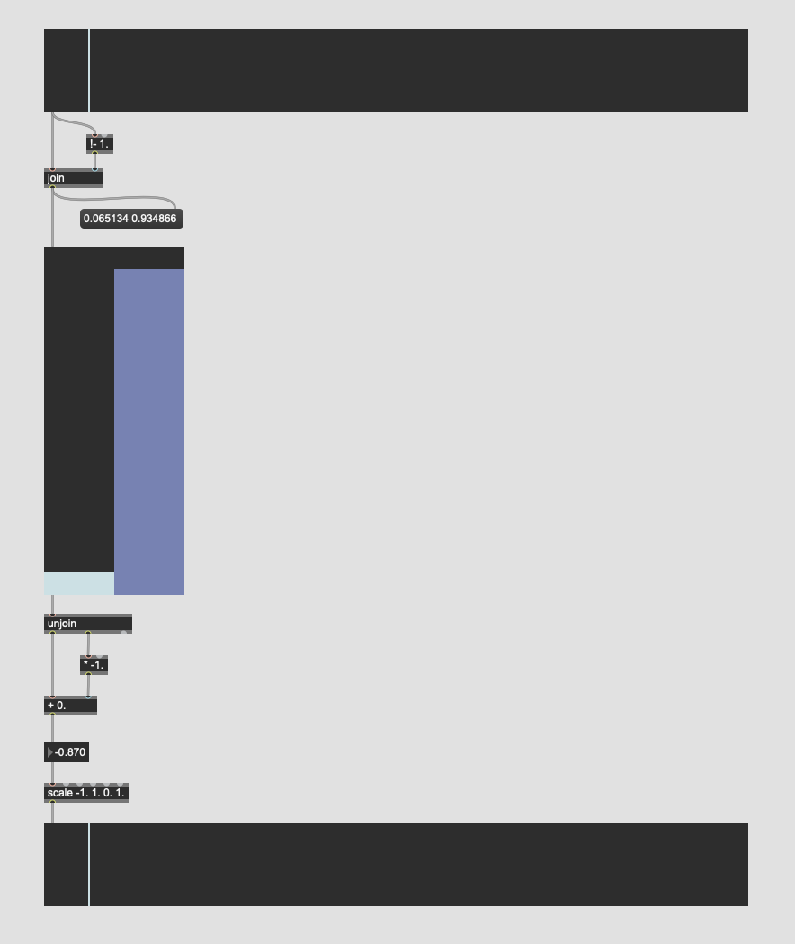
We then experimented with a few things, but found the best results by putting that into fluid.knnregressor~ with the incoming descriptors (104d MFCC soup) on one side, and the “one-hot” vector ont he other side.

This meant that when interpolating outputs based on new inputs it would give me something like:

0.951523 0.048477

This could then be operated on and turned back into a single continuous vector, representing the interpolation between the classes.

This gave us a jumping off point.

//////////////////////////////////////////////////

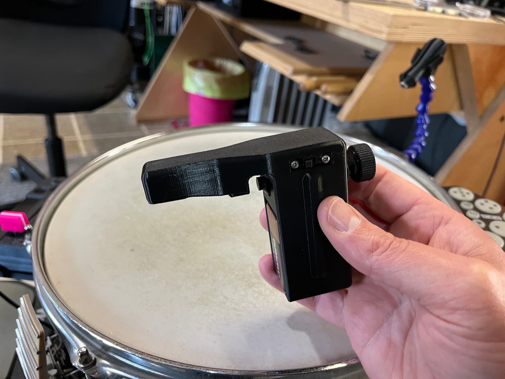
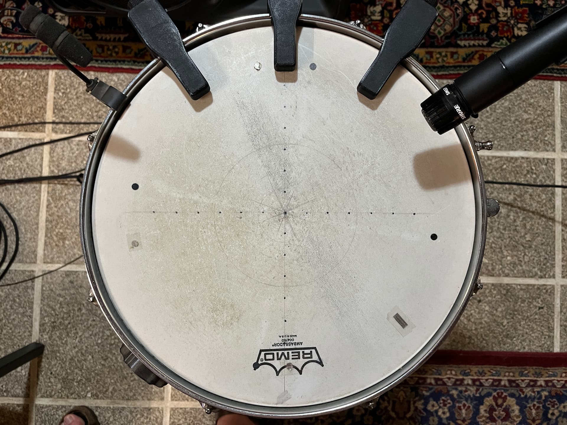
Where this fell a bit short was that although it worked alright (and loads better than things I had tried before), it would still get a bit jumpy in the middle. To mitigate that @balintlaczko suggested manually adding an explicit in-between class. So I set about creating some new training (and performance) datasets that had 2, 3, 5, and 8 classes, which was easy enough to do, as my snare looks like this these days from other experiments:

That led to these initial results:

You can kind of see this in the video, but here are the plots of the classes for each.

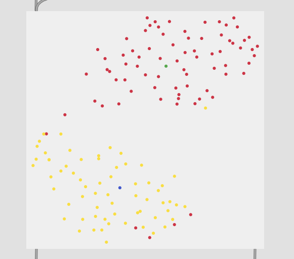
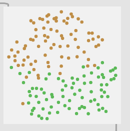
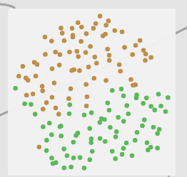
2 classes (center and edge):
2 zones

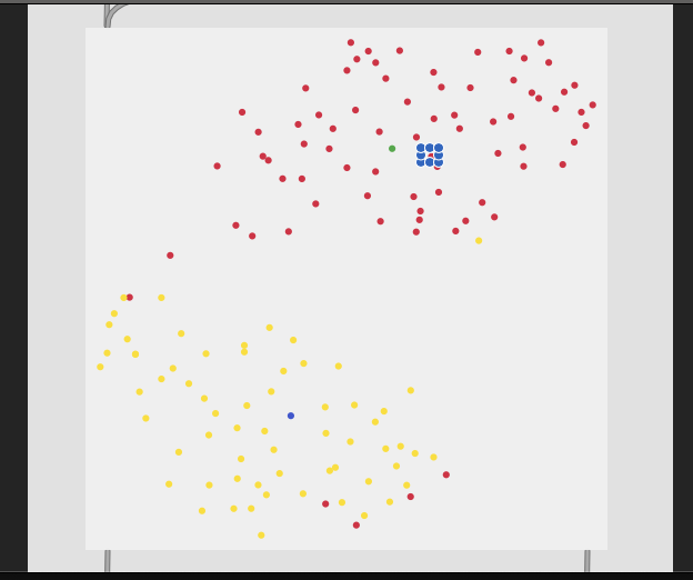
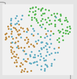
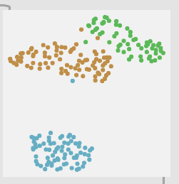
3 classes (center → middle → edge):
3 zones

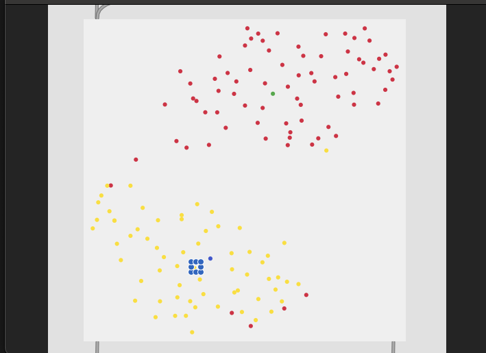
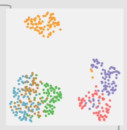
5 classes (middle bits between the middle bits):
5 zones

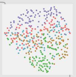
8 classes (as granular I could be with my pencil marks):
8 zones

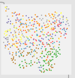
So with these you can see clear separation between the two classes in the first, then varying amount of overlap with the rest.

At this stage I think either the 3 or 5 class versions work the best.

//////////////////////////////////////////////////

I did also experiment with fit-ing fluid.mlpregressor~ in the same way, but this didn’t give good/useful results. Firstly it was really hard to train, taking a long time for anything above 3 classes (and I never got the 8 class version to converge at all) and then when it was properly fit it seemed to actually learn the “one-hot” encodings too well. Meaning that I was back to square zero where rather than interpolating between the classes, it tended to jump between them.

Here’s the vid I made showing that behavior:

//////////////////////////////////////////////////

At this point it seemed like the results were already “usable” (though not perfect) as long as you manually trained interim classes.

I still wanted to smooth out and improve the scaling a bit, so I experimented a lot with @numneighbours. I believe for the initial video I was using something quite small, ~@numneighbours 5 on a dataset where each class was ~80 entries.

I then experimented with going really far in the other direction with something like @numneighbours 80, so almost a 1:1 of neighbors to amount of entries per class and this worked a lot better. Or rather, for this use case, produced more consistent/smooth results.

I then coupled with this with some reduction in the overall range so the first class was more “0.” and the last class was more “1.”. Something like zmap 0.3 0.7 0. 1..

So far this is working pretty well, and although the 3+ class versions are a touch smoother, the 2 class versions are pretty usable as they are.

//////////////////////////////////////////////////

As a sanity check, I wanted to see how this stacked up to the interpolation you get with the native Sensory Percussion software.

I fired up the v1 Sensory Percussion software I still have installed (they did come out with a big v2 update last year) and ran the same exact audio into via TotalMix/Loopback and was surprised with the results:

The results look very similar to what I’m getting with the “one-hot” approach! (i.e. kind of jumpy, not using the whole range, etc…)

Overall it looks slightly better, but it’s not this “perfect” interpolation between the classes that I was expecting it to be.

//////////////////////////////////////////////////

So all of this up to this point has been working on the descriptor recipe that I developed/tweaked over the last few years (outlined here).

Basically this:

13 mfccs / startcoeff 1
zero padding (256 64 512)
min 200 / max 12000
mean std low high (1 deriv)

Previous to the last few weeks, the best results I had gotten was trying some stuff @weefuzzy (and @tedmoore) suggested in this thread from a few years ago. In short taking the 104d raw MFCCs and reducing it down via an automated PCA thing to keep 95% of the variability of the dataset intact.

When I had the initial zoom chat with @balintlaczko I had prepped some of this and while it worked ok, it was pretty shit. But now that we had a different/new approach, it was time to revisit combining them the approaches (“one-hot” + PCA).

I set about to do this only to realize that since I was operating on the labelset directly (to create the “one-hot” vectors), that that part of the patch/approach wasn’t impacted at all. What was impacted was what was fed into fluid.knnregressor~'s input.

While starting this up I found I got awful awful separation between the classes when using this 104d->PCA95->normalization. Check this out:

2 classes of 104d MFCCs:
2 zone

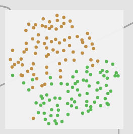
2 classes of 31d normalized PCA:
2 zone reduced

Everything is all blurry and mushed together. Although I didn’t test this data in a vanilla classification context, I would imagine it would work terribly.

After doing a bit more poking/testing, it seems that the normalization made the (reduced) MFCCs pretty erratic.

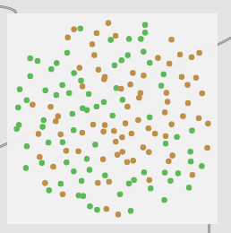
If I instead use the PCA reduced version but sans normalization, I instead get this:
Screenshot 2024-02-08 at 12.02.24 AM

Which looks functionally identical to the 104d MFCCs.

More than that, they perform almost identically:

There’s some tiny variance for some middle points, but overall it doesn’t seem to make a big impact here

//////////////////////////////////////////////////

So that takes us to present day…

I still want to test some more stuff. @balintlaczko has suggested trying some spectral descriptors/stats (rather than MFCCs) which I plan on setting up. Given how well the MFCCs tend to separate the classes in the plots above, I’m curious if this will work better, but you never know until you try.

I also still want to refine the @numneighbours “smoothing”, specifically as a ratio vs the amount-of-entries-per-class. I have a feeling that 50-100% works well for something smooth (and 2 input classes), but given more explicit middle classes, something lower is probably better (20-50%).

I also want to test it across a wider range of material. So far I’ve mainly done the center/edge classes, as these are pretty worst-case-scenario in terms of similarity. Here is a plot for rim shoulder → rim tip for example:
3 zones (rim on shoulder)

And here is a 6 class version with center/midd/edge + rimshoulder/rimmiddle/rimtip:
6 zones (center to edge and rim on shoulder)

Although I haven’t actually tested the 6 class version, the 3 class version works about the same even though the gaps in the plot are much larger.

Seeing this made me wonder about trying to incorporate a @radius-based approach in addition to (or instead of) the @numneighbours, but sadly that isn’t a possibility with fluid.knnregressor~. Perhaps by packing stuff into a fluid.kdtree~ and requesting all the nearest matches and doing the math on the manually or something. Not sure.

//////////////////////////////////////////////////

So yeah, wanted to bump this post with some info/updates. If anyone has any thoughts/suggestions, that’d be very welcome!