IQR-ing corpora

I was looking over my Example 11 thread from last year and other than it taking a while for my to re-wrap my head around all the “indices math” involved, I was struck by this workflow:

Or @tremblap’s pseudocode version:

More specifically, how much of this is applicable if rather than PCA-ing together a descriptor space, you instead manually curate a set of descriptors/stats that you use “as is” (either using something like what @tedmoore has suggested with an SVM or more recently with @tremblap’s suggestion of parsing through PCA to see the weights of given dimensions).

All of that is to say, a lot of the workflow above involves standardizing->pca->pruning->normalizing. Obviously things like loudness-weighted descriptors would still be fantastic, but if I have a fairly low (20-30) dimensional space that is made up of natural dimensions, perhaps some of this workflow isn’t necessary/desired.

At the moment I’ve been trying to build a purely fluid.kdtree~-based version of my matching and it works well if I’m using somewhat overlapping descriptor spaces, or if I would like descriptor spaces to purposefully (and unevenly) overlap. As in, I want to match loudness/pitch even if they aren’t the same in my input and corpus. But if I would like to make the spaces overlap, I know that IQR is the way to go for this. I believe that example 11 predates the inclusion of IQR in the fluid.verse~ but either way, it’s a bit tricky to figure out how to best deal with the datasets/dimensions if you want them to remain absolute (i.e. pitch matches exact pitch).

At the moment I’m mainly using the means of 20 (19) MFCCs, loudness, and pitch, as those were the most effective (natural) descriptors in my tests here, and these numbers are pretty all-over-the-place in terms of range. Since I’m analyzing/matching like-for-like I’ve just shoved them as is into fluid.kdtree~ and it seems to work fine, but I’m not entirely sure what I should be doing to improve the distance matching if I want to retain absolute descriptor spaces. And as mentioned above, what to do with IQR-ing things for when I would like to scale/normalize the spaces.

@tremblap mentioned in the thread about fluid.datasetplot~ that @weefuzzy is working on some of this stuff so hopefully this will become clearer on the weekend, but still wanted to make a thread about it here in the interim.
I think @tremblap and I had crossed wires – I’m not really working on something like this. I do indeed have a problem of disjoint spaces to think through, but not relating to interpretable features in this way.

Anyway: I get a bit lost in the above with what you actually want to happen. Could we nail it down a bit? Is it a change in what gets matched? If your corpus pitches are all (say) G4-G5, and your played data are all (say) G2-G3, what is it you’d like to be able to do?

1 Like

Sorry, was a ramble-y early morning email!

In short, it’s both. Sometimes I’d want nothing to be rescaled (so G2 would be G2, using pitch as an example), and if I have no G2s in my input, a bunch of samples in the corpus wouldn’t be used. So there’s some general workflow questions around this (G2=G2) approach in terms of what to put in the fluid.kdtree~ so matching isn’t skewed by large numbers (dB/MIDI). In Example 11, there’s loads more data munging, but I wonder how much of it is useful/desirable if there’s no fluid.pca~ in play.

The other use case would be rescaling the spaces (so G2 = F#6 or whatever), where I want to have the spaces overlap for maximum coverage. In the past I’ve done this with an abstraction that takes minimum, mean, and maximum values and makes a spline scaling around that middle point, but I believe/suspect IQR is the better choice here since it doesn’t transform the data so much. And then following on from that, there’s still the question of if there’s more data processing around that for fluid.kdtree~-ing.

If ‘wouldn’t be used’ = ‘ignored’ then this is no longer a straightforward nearest neighbour search. What would happen in a nearest neighbours search is that the results would all be pulled in the direction of G2.

If the ranges of each dimension of the data against which the tree is fitted don’t have more or less equal ranges, then queries will be weighted towards those dimensions with the greater range, as these will dominate the calculated distances between points. So, you don’t need standardise for the same reasons it’s needed in PCA (where the assumption of zero-mean, unit comparable variance is quite important), but you need something that will put different dimensions on a equal pegging (or unequal-by-design); so, that could just as well be normalised as standardised.

I think that’s simpler: standardise / scale the spaces independently of each other.

Not necessarily: it depends on the distribution of what you’re fitting. If the input really does have outliers that would yield an unhelpfully large variance when standardising, then robust scaling will help with that. But it’s predicated on the assumption that there are outliers so (I think) if the input is actually closer to normally distributed it would end up affecting the input more.

1 Like

I was getting it but this threw me:

To give a clearer example, say I’m playing only crotales on my snare, but have a corpus of concert bass drum sounds. The overlap there is not very big (in terms of timbre/pitch at least), but I may hit the crotale with a soft mallet in a way that overlaps with the descriptor space of the corpus. So in this use case, I would want those matches to be returned, but not if I’m playing twinkly twinkly sounds.

So not explicitly ignoring things as such, but perhaps setting the @radius of fluid.kdtree~ to something small enough that it just doesn’t match it.

Is that not a straightforward nearest search (with nothing nearby)?

I guess what was confusing me here is that there may be a generic standardization/scaling that is applied (for the distance matching) that is (I guess?) independent of any scaling of the two descriptor spaces to each other.

As in, if I want to match according to my (non-overlapping) crotale/bassdrum example above, you’re saying I should still stand/scale the descriptor space, but I guess applying the same fit to both, so they are relative to each other in terms of absolute numbers (e.g. G2 = G2).

BUT

If I want to make those spaces overlap, I would still stand/scale things, but independently of each other so the spaces overlap maximally.

I guess a third example/usecase here is where both are independently standardized, but then arbitrary scaling is applied (e.g. the crotales input is scaled down so it only covers the very dry/muffled sounds in the bass drum corpus (e.e.g.g. if both are normalized to 0. to 1., the crotales would be re-rescaled to cover only 0. to 0.3)).

Adding radius will work (probably) but IMO is less straightforward than just calling `knearest’ with the default radius = 0 (which would always return something). So long as we’re clear that the search will still, essentially, be dragged in the direction of whatever pitch in the tree is nearest your bandit (so I reckon the results would be different from ignoring it altogether).

Yes. Scaling and shifting your input (especially w/r/t to a predictable and consistent range in the tree) can be really useful for controlling the homogeneity or otherwise of what’s coming out.

1 Like

Ok, revisiting this today.

So first the noob-y question. Does IQR-ification happen inside fluid.bufnormalize~? (e.g. @min 0.25 @max 0.75?) According to the helpfile that’s the output range, and if I’m understanding correctly, you want the input to be used to compute the IQR-ing.

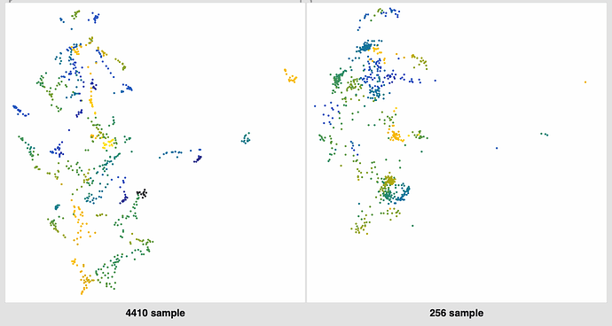
Now, only a cool thing that @tedmoore suggested ages ago, that I only finally got around to now. For my Time Travel stuff, Ted suggested a sanity check to see if the descriptors from 256 samples are even in the same ballpark as what you get from 4410, or more specifically, if you can (somewhat) accurately predict a 4410 window with only 256 samples (given a finite, and predefined set of inputs).

I had been putting this off as I had no (easy) way to visualize stuff, but that’s sorted now.

Before I get on to the question(s) stuff, here are the results of my first test with this.

This is feeding the same audio into the same process (I think (more on this below)) and then plotting them in the same reduced (umap) space.

The results look pretty good actually. Not perfect, but not completely incompatible.

So my process here was to take a 42d space (20MFCCs(19), loudness, pitch, with mean/std of everything) then standardize, umap, normalize, then plot.

My question is with regards to doing a workflow like this to see how things overlap in an absolute sense.

What I did here was run that process (standardize->umap->normalize) on the 4410 dataset, then write the fits for those three objects/processes to disk, then load up the 256 sample version, read all those .jsons, then transform (instead of my initial fittransform).

Is that correct?

And as a follow up. If I understand @weefuzzy’s previous posts correctly, other than figuring out where the IQR stuff fits in, if I wanted to force the overlap between these descriptor spaces I would independently standardize/umap/normalize? Or would I keep the same umap-ing, so things kind of relate?

(as an aside, my intended workflow at the moment is to not use UMAP/PCA at all in the processing, other than for visualization, but still want to wrap my head around this side of things)

I saw @pasquetje mention it in the other thread. It’s the sneakily named fluid.robustscale~!

1 Like

Actually, I’m not sure what the difference between fluid.standardize~ and fluid.robustscale~ is (in terms of behavior). fluid.standardize~ gives you a standard deviation as -1/1 and in fluid.robustscale~ you can set similar behavior via what you set the centiles to, but both are center mean-ing processes no?

I guess the names are mathematically significant (“standardizing” vs “robust scaling”). Is that the main distinction? Otherwise it seems like it’d be great to have these kinds of things be the same object where you can set the distance in deviations or centiles or something, but I guess that’s not the flavor of TB2 at all.

If I am not wrong, fluid.standardize~ is taking count of the mean while fluid.robustscale~ is taking count of the median.

fluid.standardize~ contains the information for all the values thanks to the mean. This makes it easier to separate/compare values. The barycenter of dataset will not always in the center of the space.
Values from fluid.robustscale~ contain the information of the center value so it is easier to see the value/position of each point relative to the “center point”. The barycenter of dataset remains at the center of the space.
Topology differs.

Tell me if I am wrong…

2 Likes

bufnormalize?

We can talk - but outliers at the moment can be removed in a time series (in bufstats) only. In robustscale it is not removed but not considered in the range (see below)

This is exact. Let me go a bit verbose:

  • for each dimension independantly, each do the same thing: they try to fit the data within a predictible range.
  • standardise centres on 0 the mean (average) of the dimension, and will make +/- 1 standard deviation align with +/-1. This works well with data that has a normal distribution. For much of our stuff, it is not true, so we need…
  • robust scale centres on 0 the median (the middle value of that dimension) and makes the +/-1.0 range fit + and - the interquantile range. So -1 to +1 will cover a window of twice the distance of the middle 50% of your data. That might be all of it. That might not. There is no control on this. You just know that at least 50 % of your data will be within that range for sure.

Because a graphic explains it all better than me I recommend the helpfiles and to try to guestimage the values with simple arrays. In the tutorial file I’ve done that with 10 items which I find ideal to see where average and standard deviation fail, and where robust scaling helps give more useful information.

Then there are the scikit learn pictures which are always good.

1 Like

That was a typo. I was on a posting spree, so crossed my wires between the different hierarchies of data storage (buffers/datasets).

My maths aren’t good enough to know, but isn’t +/- a deviation also specify that it covers some kind of percentage of the data? I’m guessing there’s a more significant distinction between deviations and centiles here, but to ask the question in a kind of different way. Can you get the same results out of standardization and robust scaling (if you ignore the mean/median distinction)? Specifically with regards to % of the data that is contained within +/-1.

Some helpfile tabs would be super useful to demonstrate these distinctions though (with diagram/datasets ala that webpage) since I wouldn’t have thought to look for something called “robust scaling” if I didn’t know what that meant mathematically.

I noticed :heart:

The problem here is that explaining maths without doing maths is quite hard. I’ll try to devise examples but I think that the IQR explanations of Khan Academy are quite approachable and graphic enough… let me know if they help. Otherwise I’ll try to devise some of them for our user pool…

https://www.khanacademy.org/math/statistics-probability/summarizing-quantitative-data/variance-standard-deviation-population/v/mean-and-standard-deviation-versus-median-and-iqr

1 Like

8 minutes of youtube, with a clear explanation of when average and std fail us.

Only if the data is normally-distributed (in which case ±1 standard deviation() accounts for 68% of the observed sample, 95% within two, 99.7% within three). But only if it’s normally-distributed.

2 Likes

That’s the main distinction I think. I understood it to force the data into those percentages in the first place. But I guess it just draws the lines, and the data falls where it falls(ish).

We cannot stress this enough. The Khan 8 minute video is very very hands-on to show how it is sooooo problematic an assumption for asymmetrical data like most of mine.

1 Like

Cool, yeah that makes sense.

So is the idea then, with a “normal” (0.25/0.75) IQR that you still use/map/whatever the data points above/below the +/-1 you get, or is it (typically) the case that a separate clamping (or pruning) process is applied?

Obviously every case is different, but in a typica or best practice way.

This question is again complicated. Did you check the Khan movie above?

I’ll try to devise a very concrete example here. It is a verbose math version of the audio example of pitch analysis in the example folder - example 10b

We have pitch here, and because of attack and windowing and noise, the frames look like this, in midi cents.

96.9, 50.1, 50.2, 100.1, 50.0, 50.2, 96.9

the extreme frames are non-descript (in our case, nyquist/10, which is 96.9024 at 44100) and there is one (classic) octave jump at one point. You get:
mean 70.6
stddev 23.7
values within +/- 1 std of mean: [50.1, 50.2,50.0, 50.2]
median 50.2
IQR 46.7
values within ±/ 1 IQR: [96.9, 50.1, 50.2, 50.0, 50.2, 96.9]

Advantage of median vs mean: value is from the set - it actually exists.
The advantage of IQR is more ambiguous: the default value of the pitch becomes problematic as it is in the range of significant values here, which is a good case once more to change it (it will happen one day) but at least it keeps the problem - this is why we have pitch confidence removal as an option but let’s not digress - we’ll give that example below.

Just for shits and giggles, let’s use @a.harker descriptor, which throws 0s instead of potentially valid value for the non-descript pitches:

0, 50.1, 50.2, 100.1, 50.0, 50.2, 0

mean: 42.94
stddev: 31.99
values within +/- 1 std of mean: [50.1, 50.2,50.0, 50.2]
median: 50.1
IQR: 25.2
values within ±/ 1 IQR: [50.1, 50.2, 50.0, 50.2]

the mean is still insignificant, the median still valid. The IQR is still intersting. the values passed through seem better but they are on wrong grounds. Let’s remove invalid values via a quality assessment, which we can do, via thresholding pitch confidence (or loudness or whatever you care)

50.1, 50.2, 100.1, 50.0, 50.2

mean: 60.1
stdev: 20.0
values within +/- 1 std of mean: [50.1, 50.2,50.0, 50.2]
median: 50.2
IQR: 0.1
values within ±/ 1 IQR: [50.1, 50.2, 50.2]

Again, mean and std dev give you strange values which, like in the Khan example, do not seem to relate to our data distribution too much. It is because they assume standard distribution, which we rarely have in our type of small curated data.

I hope this helps a bit. I recommend trying to check and understand example 10b.

1 Like

I did watch the video and it helped clarify how that can be better for misshapen (non gaussian) datasets.

I remember going through that patch a bit ago, though it would be worthwhile revisiting with IQR at hand, as I struggled pulling out the most useful information there before for reasons as you’ve outlined here.

I guess, in general, it’s still useful knowing “best practice” stuff as training wheels of sort, as it’s (near) impossible trying to learn anything where the answer is “become a data scientist”. Or to use a more concrete metaphor (which I may have mentioned on a Thursday geekout) where I’m trying to learn to tune a guitar, and we end up talking about 8 string early instrument intonation approaches as applied to contemporary classical music interpretation etc… Maybe it’s useful to know that the first string should be tuned to E, then build from there.