Regression + Classification = Regressification?

rodrigo.constanzo · May 12, 2022, 3:07pm

Ok, I got to some coding/tweaking and made a lofi “automatic testing” patch where I manually change settings and start the process, then I get back quantified results (in the form of a % of accurate identifications).

I’m posting the results here for posterity and hopeful usefulness for others (and myself when I inevitably forget again).

My methodology was to have some training audio where I hit the center of the drum around 30 times, then the edge another 30-40 times (71 hits total), then send it a different recording of pre-labeled hits. These were compared to the classified hits and a % was gotten from that.

Given some recent, more qualitative, testing I spent most of my energy tweaking and massaging MFCC and related statistical analyses.

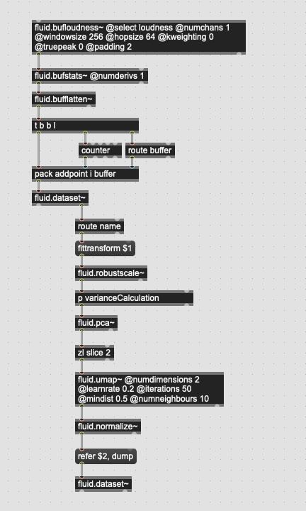
All of this was also with a 256 sample analysis window, with a hop of 64 and @padding 2, so just 7 frames of analysis across the board. And all the MFCCs were computed with (approximate) loudness-weighted statistics.

//////////////////////////////////////////////////////////////////////////////////////////////////////////////////

To save time for skimming, I’ll open with the recipe that got me the best results.

96.9%:

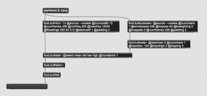
13 mfccs / startcoeff 1
zero padding (256 64 512)
min 200 / max 12000
mean std low high (1 deriv)

//////////////////////////////////////////////////////////////////////////////////////////////////////////////////

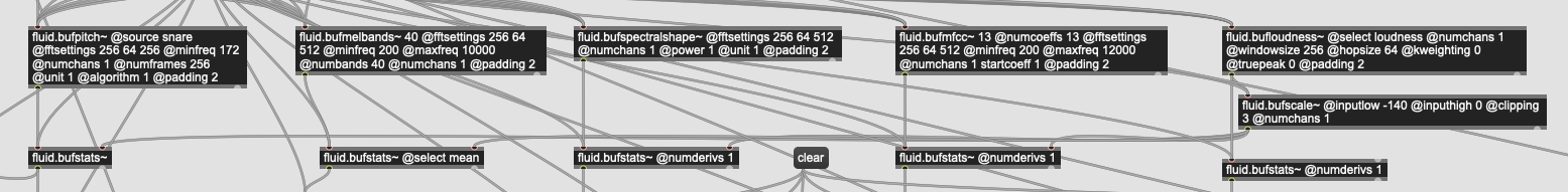
As mentioned above, I spent most of the time playing with the @attributes of fluid.buffmfcc~, as I was getting worse results when combining spectral shape, pitch, and (obviously) loudness into the mix.

I remembered some discussions with @weefuzzy from a while back where he said that MFCCs don’t handle noisy input well, which is particularly relevant here as the Sensory Percussion sensor has a pretty variable and shitty signal-to-noise ratio as the enclosure is unshielded plastic and pretty amplified.

So I started messing with the @maxfreq to see if I could get most of the information I needed/wanted in a smaller overall frequency range. (still keeping @minfreq 200 given how small the analysis window is)

83.1%:

20 mfccs / startcoeff 1
zero padding (256 64 512)
min 200 / max 5000
mean std low high (1 deriv)

81.5%:

20 mfccs / startcoeff 1
zero padding (256 64 512)
min 200 / max 8000
mean std low high (1 deriv)

93.8%:

20 mfccs / startcoeff 1
zero padding (256 64 512)
min 200 / max 10000
mean std low high (1 deriv)

95.4%:

20 mfccs / startcoeff 1
zero padding (256 64 512)
min 200 / max 12000
mean std low high (1 deriv)

92.3%:

20 mfccs / startcoeff 1
zero padding (256 64 512)
min 200 / max 14000
mean std low high (1 deriv)

92.3%:

20 mfccs / startcoeff 1
zero padding (256 64 512)
min 200 / max 20000
mean std low high (1 deriv)

What’s notable here is that the accuracy seemed to improve as I raised the overall frequency range with a point of diminishing returns coming at @maxfreq 12000. I guess this makes sense as it gives a pretty wide range, but then ignores all the super high frequency stuff that isn’t helpful (as it turns out) for classification.

//////////////////////////////////////////////////////////////////////////////////////////////////////////////////

I then tried experimenting a bit (somewhat randomly) with adding/removing stats and derivatives. Nothing terribly insightful from this stream other than figuring out that 4 stats (mean std min max) with 1 derivative of each seemed to work best.

92.3%:

20 mfccs / startcoeff 1
zero padding (256 64 512)
min 200 / max 12000
mean std (no deriv)

93.8%:

20 mfccs / startcoeff 1
zero padding (256 64 512)
min 200 / max 12000
mean std (1 deriv)

90.8%:

20 mfccs / startcoeff 1
zero padding (256 64 512)
min 200 / max 12000
all stats (0 deriv)

90.8%:

20 mfccs / startcoeff 1
zero padding (256 64 512)
min 200 / max 12000
all stats (1 deriv)

//////////////////////////////////////////////////////////////////////////////////////////////////////////////////

Then, finally, I tried some variations with a lower amount of MFCCs, going with the “standard” 13, which led to the best results, which are also posted above.

83.1%:

13 mfccs / startcoeff 1
zero padding (256 64 512)
min 200 / max 5000
mean std low high (1 deriv)

96.9%:

13 mfccs / startcoeff 1
zero padding (256 64 512)
min 200 / max 12000
mean std low high (1 deriv)

//////////////////////////////////////////////////////////////////////////////////////////////////////////////////

For good measure, I also compared the best results with a version with no zero padding (i.e. @fftsettings 256 64 256), and that didn’t perform as well.

93.8%:

13 mfccs / startcoeff 1
no padding (256 64 256)
min 200 / max 12000
mean std low high (1 deriv)

//////////////////////////////////////////////////////////////////////////////////////////////////////////////////

So a bit of an oldschool “number dump” post, but quite pleased with the results I was able to get, even if it was tedious to manually change the settings each time.

tedmoore · May 13, 2022, 2:35pm

I love this.

rodrigo.constanzo · May 26, 2022, 11:32am

Ok, so I’ve finally pushed this a bit further and have tried getting into the nitty-gritty PCA->UMAP-type stuff.

Took me a bit of hoop jumping to get there, but finally was able to test some stuff out.

So as a reminder/context, I’m trying to analyze realtime audio with a tiny analysis window (256 samples) and then feed that into a regressor to “predict” what the rest of that sound would sound like.

I’m doing this by building up two datasets of the same sounds. The first one being the first 256 samples, and the second being the first 4410 samples (I may experiment with this being samples 257-4410 instead).

I have a few premade hits of me playing snare with various sticks/techniques/dynamics/objects/etc… I’m testing things with 800 hits, though I can see myself going much higher than that for a comprehensive version (and also much lower for a quick-and-dirty-borrowed-snare context).

//////////////////////////////////////////////////////////////////////////////////////////////////////////////////

I spent the bulk of the time trying to create an analysis workflow similar to what I was doing with my LTE idea (adapted from @tremblap’s LPT idea) where I funnel each “high level” descriptor through its own processing chain, with the idea of ending up with a lower dimensional space that represents the higher dimensional space well.

For the sake of simplicity/testing, I did: Loudness, MFCCs, SpectralShape, and Pitch. Quite a bit of overlap there, but it’s easier to test this way then trying to piecemeal things like I was doing in the LTEp patch.

The actual patch is quite messy, but each “vertical” looks something like this:

And the top-level descriptor settings are these:

(the melband analysis is for spectral compensation that runs parallel to this)

At the bottom of this processing chain is a bit that puts all the fluid.dataset~s together, and saves the fits for everything.

//////////////////////////////////////////////////////////////////////////////////////////////////////////////////

I then tried mapping the spaces onto each other, keeping the fits the same, based on @tedmoore’s suggestion a while back. I could have sworn I did this successfully ages ago, but the results now were pretty shitty.

Here is the bottom of each processing chain with a 256 sample analysis window:

(pitch is obviously not great as these are mainly drum sounds)

And here is the 4410 sample versions, with the same fits:

(ignore the combined one on the left, as I didn’t save the fit when doing this as it’s elsewhere in the patch)

I was a bit bummed out about this as I was working under the assumption that each side of the regressor should be able to map onto each other naturally. I was reminded that this isn’t the case when rewatching @tedmoore’s useful video last night:

I guess the whole idea is that the numbers on either side don’t have a clear connection, and it is the regressor that has to create one.

//////////////////////////////////////////////////////////////////////////////////////////////////////////////////

Now over the last few days I’ve been playing with fluid.mlpregressor~. I still find this profoundly confusing as nothing ever converges, the settings are opaque, the documentation/reference is thin, and I’ve forgotten all the “common practice/lore” stuff that’s been said on the forum over the years.

Other than doing a test/simple thing (e.g. the help patch), I don’t think I’ve ever successfully fit something! (well, barring the details below).

So at first I tried feeding the results of the robustscale->PCA->UMAP->normalize processing chain and was getting dogshit results. My loss was typically in the 0.3-0.4 range.

That was using fluid.mlpregressor~ settings of:
@hiddenlayers 3 @activation 1 @outputactivation 1 @batchsize 1 @maxiter 10000 @learnrate 0.1 @validation 0

I would run that a handful of times, and the numbers would go down slightly, but not by any meaningful amount. They would also sometimes go up.

After speaking to @jamesbradbury he said that that was probably an ok amount of loss since the amount of points/data is pretty high (8d with 800 entries).

On a hunch, I decided to try something different this morning and instead feed the network 8 “natural” descriptors. As in, mean of loudness, deriv of mean of loudness, mean of centroid, etc… So 8 “perceptual” descriptors, with no post processing (other than normalization so they would fit the @activation 1 of fluid.mlpregressor~. That instantly got me better results.

I tried again using only 6 descriptors (leaving out pitch/confidence) and that was even better!

Here are the results of the tests I did, along with the network size, and what was fit first:
@hiddenlayers 3
6d of natural descriptors (no pitch): 0.096001
8d of natural descriptors: 0.160977

8d of pca/umap (256 fit): 0.325447
8d of pca/umap (4410 fit): 0.463417

@hiddenlayers 4 2 4
6d of natural descriptors (no pitch): 0.092399
8d of natural descriptors: 0.155284

8d of pca/umap (256 fit): 0.317485
8d of pca/umap (4410 fit): 0.44022

//////////////////////////////////////////////////////////////////////////////////////////////////////////////////

This was pretty surprising I have to say. If it holds up (I’ve run the tests twice and it has), it would be even more useful for my intended use case (analyzing “long” windows in “realtime”) since the numbers on either side “make sense” and are relatively scalable. As in, I know what the mean of loudness is, and can do something with that from the predicted version, as opposed to 1d of a slurry of PCA/UMAP soup.

I still need to have a think on what I want to do with the results of the regressor as my idea, presently, is to use that to find the nearest match using fluid.kdtree~, with the idea being that with the longer analysis window I can have a better estimation of morphology (and pitch). That being said, it is a predicted set of values, rather than analyzed ones, so I’d want to weigh them accordingly, something I’m not sure how to do in the fluid.verse~.

Additionally, I’m not sure what descriptors/stats make the most sense to match against. Perhaps some hybrid where I take “natural” descriptors for loudness/pitch, but then have a reduction of MFCCs in the mix too? I do wish fluid.datasetquery~ was easier to use/understand, as I could just cut together what I want from the datasets below, but each time I go to use it I have to spend 5 minutes looking through the helpfile, and then another 5 figuring out why it didn’t work, and another 5 making sure the actual data I wanted was moved over once it does work.

//////////////////////////////////////////////////////////////////////////////////////////////////////////////////

SO

I welcome thoughts/input from our resident ML gurus on things that could be improved/tested, or the implications of having “natural descriptors” regressing better than baked/cooked numbers.

//////////////////////////////////////////////////////////////////////////////////////////////////////////////////

Here are the datsets I did my testing with if anyone wants to compare/test.

NATURAL_6d.zip (113.7 KB)
NATURAL_8d.zip (113.7 KB)
PCA_UMAP_256fit.zip (123.9 KB)
PCA_UMAP_4410fit.zip (123.9 KB)

weefuzzy · May 26, 2022, 4:20pm

@tedmoore and @jamesbradbury are hard at work developing considerably better docs but I think you know that.

Some important aspects of lore that we’ve discussed at various points

absolute loss numbers aren’t all that important, and they don’t by themselves signify convergence or not. They’re especially meaningless for regressors without reference to the number of output dimensions and the range of each of those dimensions
accordingly, the way to work when adjusting the network for a task is to use a small number of iterations and repeated calls to fit and look at the loss curve over time.
even then, the litmus test of whether a network is working as desired is not how well it does in training but how well it does with unseen test data (and even then, you might just have a ‘clever horse’)
if things aren’t converging then the learning rate is probably too big, but maybe too small: an important initial step is to find the point where it becomes noisy in the loss curve and back off from there
a batchsize of 1 will likely result in noisier convergence
the number of in / out dimensions isn’t the only important thing when working out if you have enough data: what you need to think about is the number of unknown parameters the network is learning, which is a function of the dimensionality at each layer
the quantity of data needs to be matched by the quality as well. Starting with a small number of raw descriptors is a perfectly sensible thing to do. Whether they exhibit patterns that match what you want the network to be sensitive to needs to be established empirically (i.e look at the descriptors over time and see if they (some of them) wiggle at points where you need to see wiggling). Being parsimonious is also a good idea: stuffing the learning process with loads of derived stats etc. is unlikely to help things if those stats don’t increase the obviousness of the things you want to capture.