Regression + Classification = Regressification?

Ok, did some more testing (and my original dataset, to keep things consistent) and it’s a bit weird.

So it looks like the 67% results I got were from using just 13 MFCCs, which I have since moved on from. And it also turns out I think I was compiling the stats from the 2nd derivs wrong (more on this below).

Results are a bit surprising too.

So this is run with a 10point training set, and then fed 50 random samples where there are 5 of each “type” present in the original training set (i.e. 5x snare center, 5x cross stick, etc…).

I run this 1000 times, and see how often both of the values were the same. I also ran this whole process three separate times, making sure to close/open everything again between each run.

20MFCCs with 1 derivative: 76.1% / 76.7% / 75.8% = 76.20%
25MFCCs with 1 derivative: 71.7% / 75.9% / 72.4% = 73.33%
25MFCCs with 2 derivatives(?): 73.1% / 72.1% / 74.0% = 73.07%

A couple of striking things here. It turns out my results got worse with the higher MFCCs count. I think the matching with the 2nd derivative with 25MFCCs is better, but the numbers got skewed with an outlier for the second test of 25MFCCs with 1deriv.

I haven’t run the 20MFCCs with 2derivs yet, because I think I’m fucking something up in terms of creating the dataset/entry.

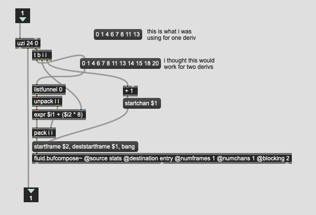
Up to this point I’ve been using an adapted version of @tremblap JIT-MFCCs code for unpacking and flattening the fluid.bufstats~ stuff. (I know we have fluid.buf.select and fluid.bufflatten~ but the js inside fluid.buf.select means it won’t fare too well for fast/real-time use).

So to adapt this code to 25MFCCs (sans 0th coefficient) I changed the uzi and that does it. I thought I understood the list bit, where it’s taking the mean, standard deviation, min, and max for the original stats and then +7 everything to do the same for the derivatives.

Screenshot 2020-07-27 at 1.59.48 pm

But something isn’t adding up right.

If I run this process with 20MFCCs and 1deriv I get 152 dimensions. If I adjust things to get 2 derivs, I then get…156 dimensions. Which leads me to believe somethings gone fucked.

Same goes for 25MFCCs. With a single deriv I get 192d, and if I change to 2derivs I get 196d.

Have I misread that bit of patch?

the problem is in the expr (you still have an offset of 8)

what you need to do is to really understand that patch with a dummy buffer in and check what you get at the output. The problem of interface would be a solution you would have even more (imagine bufstats with binary inputs like you laughed at me in the other thread on the exploration patch) but there is very little leeway in designing options of what stats you get out otherwise…

Aaah.

So would I need to offset 8 and 16?

I’d be down with a bufstats where you only get what a you ask for if that’s what you mean! (I don’t doubt that I would have razzed about something but I was surprised that all the spectral stuff and stats returned everything no matter what)

I’ve tried making sense of this patch fragment, it’s just really gnarly and doesn’t adapt well. Adding more MFCCs was easy enough but derivs is a pain.

no. if you have 8 items in the list in the code you plunder and there is an 8 in the expr, I reckon that if you put 12 items, you’ll need to multiply by 12 in the expri

1 Like

Gotcha!

Duh, lol.

I figured out the other numbers 12 was 13-1, etc… but I was looking at the 8 and was thinking “what is this number related to?!”.

1 Like

Ok, thanks to @tremblap’s helpful comments about that patch nugget, I’ve done some proper testing and comparing between all the variables at hand (pre-reduction).

The corrected and updated stats are:

20MFCCs with 1 derivative: 76.1% / 76.7% / 75.8% = 76.20%
20MFCCs with 2 derivatives: 76.6% / 73.6% / 75.0% = 75.07%
25MFCCs with 1 derivative: 71.7% / 75.9% / 72.4% = 73.33%
25MFCCs with 2 derivatives: 69.7% / 69.1% / 67.9% = 68.90%

So, surprisingly the 20MFCCs with no addition derivatives works out the best, with the 2 derivatives being only a touch behind. Surprisingly having 25MFCCs wasn’t better. Perhaps the extra resolution in this context isn’t beneficial and/or it’s capturing more noise or something else.

@weefuzzy’s intuition about the reduced usefulness of 2nd derivatives for such short analysis frames is correct.

I’m now tempted to try min-maxing the raw MFCCs and/or other stats to see if I can get better raw matching here, but it just takes a bit of faffing to set up each permutation to test things out.

In all honesty, 76% is pretty good considering how similar some of these sounds are (snare center vs snare edge), so it will likely do the job I’m wanting it to do. I’ll retest things once I have a larger and more varied training/testing set (with much more different sounds), but my hunch is that the matching will improve there. We’ll see.

I also now need to test to see how small I can get the PCA reduction while still retaining the best matching.

Well, well, well. What’s a data-based post without a little completionism.

So I wanted to go back and test stuff just using melbands (like @weefuzzy had suggested ages ago for the JIT-regressor stuff).

So using the same methodology as above (10 training hits, 1000 tries with testing data) but with some different stats. For all of these I’m using 40 melbands between 100 and 10k, with the only stats being mean and standard deviation.

Here are the results:

40mel with 1 derivative: 70.9% / 73.2% / 76.1% / 73.3% = 73.38%
40mel with 0 derivatives: 68.9% / 67.0% / 66.8% = 67.57%

The results are pretty good, though not as good as the MFCC-based results.

Based on the fact that I got pretty decent results from taking only the mean and standard deviation (rather than also taking min and max), I reran some of the earlier tests with 20MFCCs.

The results are pretty good, though not quite as good as taking more comprehensive stats.

Here are 20MFCCs with only mean and standard deviation as the stats:

20MFCCs with 1 derivative: 73.7% / 71.0% / 73.8% = 72.83%
20MFCCs with 0 derivatives: 71.7% / 71.3% / 73.0% = 72.00%

Where this starts getting interesting is that although the accuracy is lower, I’m getting pretty decent results with much less overall dimensions. For example, the last test there gives me 72% matching, using only 38 dimensions. As a point of reference, the best results I posted in my previous post was 76.2% which took 152 dimensions to achieve.

So it will be interesting to see how these shape up with some PCA applied, as it will be a balance between accuracy and speed, and the initial amount of dimensions for taking only mean/std is already at 25% the overall size, before any compression.

And today’s experiments have been with dimensionality reduction, and using a larger training/testing data set.

Off the bat, I was surprised to discover that my overall matching accuracy went down with the larger training set. I also noticed that some of the hits (soft mallet) failed to trigger the onset detection algorithm for the comparisons, so after 1000 testing hits, I’d often only end up with like 960 tests, so I would just “top it up” until I got the right amount. So it’s possible that skewed the data a little bit, but this was consistent across the board. If nothing else, this should serve as a useful relative measure of accuracy between all the variables below.

I should mention at this point that even though the numerical accuracy has gone down, if I check and listen to the composite sounds it assembles, they are plausible, which is functionally the most important thing here.

///////////////////////////////////////////////////////////////////////////////////////////////////////////////////////////////

So I did just some vanilla matching as above, but with the larger training set, just to get a baseline. That gave me this:

20MFCCs with 1 derivative: 44.1% / 45.5% / 46.5% = 45.37% (152d)
20MFCCs with 2 derivatives: 42.5% / 47.1% / 44.0% = 44.53% (228d)

(also including the amount of dimensions it takes to get this accuracy at the end)

I also re-ran what gave me good (but not the best) results by only taking the mean and standard deviation (whereas the above one also includes min and max).

That gives me this:

20MFCCs with 0 derivatives: 52.2% / 53.0% / 53.5% = 52.90% (38d)
20MFCCs with 1 derivatives: 54.5 / 53.0% / 52.5% = 53.33% (76d)

What’s interesting here is that for the raw matching power (sans dimensionality reduction), I actually get better results with only the mean and std. Before this was close, but the larger amount of statistics and dimensions were better.

///////////////////////////////////////////////////////////////////////////////////////////////////////////////////////////////

What I did next was test these variations with different amount of PCA-ification. This can go a lot of different ways, so I compared all of them with heavy reduction (8d) and medium reduction (20d) to see how they faired, relatively. (granted there are different amounts of dimensions to start with, but I wanted to get a semi-even comparison, and given my training set, I can only go up to 33d anyways).

As before, here are the versions that take four stats per derivative (mean, std, min, max):

20MFCCs with 1 derivative: 22.5% (8d)
20MFCCs with 1 derivative: 23.1% (20d)
20MFCCs with 2 derivatives: 26.5% (8d)
20MFCCs with 2 derivatives: 27.7 (20d)

I then compared the versions with only mean and std:

20MFCCs with 0 derivatives: 28.5% (8d)
20MFCCs with 0 derivatives: 26.2% (20d)
20MFCCs with 1 derivative: 25.5% (8d)
20MFCCs with 1 derivative: 23.0% (20d)
20MFCCs with 1 derivative: 30.0% (33d)

Even in a best case scenario, of going from 38d down to 20d, I get a pretty significant drop in accuracy (52.9% to 26.2%).

///////////////////////////////////////////////////////////////////////////////////////////////////////////////////////////////

So with all of this in mind, I get the best overall accuracy while taking speed into consideration is taking only mean and std of 20MFCCs with zero derivatives which gives me 72.0% with the smaller data set and 52.90% with the larger data set, with only 38 dimensions.

I was hoping to see if I could smoosh that a little, but it appears that the accuracy suffers greatly. I wonder if this says more about my tiny analysis windows, the sound sources + descriptors used, or the PCA algorithm in general.

My take away with all of this is to get the best accuracy (if that’s important) with the lowest amount of dimensions possible, on the front end, rather than gobbling up everything and hoping dimensionality reduction (PCA at least) will make sense of it for you.

For a use case where it’s more about refactoring data (i.e. for a 2d plot, or a navigable space ala what @spluta is doing with his joystick), then it doesn’t matter as much, but for straight up point-for-point accuracy, the reduction stuff shits the bed.

(if/when we get other algorithms that let you transformpoint I’ll test those out, and same goes for fluid.mlpregressor~ if it becomes significantly faster, but for now, I will take my data how I take my chicken… raw and uncooked)
have you tried 20 Melbands? just for fun?

I haven’t.

I’ll give a spin. I used 40 for a couple reasons. One was that I figured more bands would be better, but also it’s the amount of bands I’m already getting for the spectral compensation stuff, so that analysis comes “for free”.

Ok, tested it with 20 melbands, only mean and std, no derivatives:

20mel with 0 derivatives: 48.6%

Which puts it smack in the middle of of the 20MFCC tests where 4stats was slightly worse than this, and 2stats was slightly better.

So “ok” results, but not great.

wait, what freq range did you use to spread the 40? I presume you could use the 20 mfccs of the middle of the 40 you have already to test. if you focus on the range in which the spectrum changes, you’ll have better segregations… or maybe using PCA to go from 40 to 20 here makes more sense.

I was going from 200 to 10k for the range (for both the 40 and 20 band versions).

I think I did a bit of testing with this for the spectral compensation stuff and the 40 bands in that range worked well for applying spectral compensation. That is to say, that range and amount of bands, showed a decent amount of resolution. That may or may not directly translate to differentiation for the purposes of matching though.

I think I also tried having a more compressed set of bands “in the middle”, but with how little my analysis window is, and how much high frequency information there is with the drums/percussion/metal stuff, I think having resolution higher up was more useful in that context.

I went just now to test to see how the 20MFCCs with only mean and std (38d) fares with only a tiny amount of PCA (going down to 33d) and the results aren’t great either. The accuracy drops from 52.9% to 9.6%(!!).

So I think it’s a matter of either MFCCs not being linear (though from what @groma said during the plenary, I thought that was the case), or the relationship between the various MFCCs and stats not being linear as to make PCA not very useful for reducing data there.

Do you think melbands are better suited to this? I guess once you start taking arbitrary statistics, any input data loses some of its linearity (?), so PCA would, again, start to suffer.

I really don’t know. @groma is the boss r.e. stats and stuff, and @weefuzzy is good too… but I often get ‘it depends’ because it seems to be true!

1 Like

Yeah.

In this case all the testing is pointing to MFCC + PCA = :frowning:, though happy to test some other permutations or insights they might have.
A little bit of an update on this.

Following some super awesome help and thoughts from @jamesbradbury by testing some permutations in his FTIS I decided to try a different approach. All of my testing so far has been primarily quantitative. Literally checking how well stuff matched, to try to minmax the best results with what I could manage.

@jamesbradbury set up a thing where it would play the test audio and then the nearest match audio, so you could hear them back to back. This was useful, so we decided to go full on and implement a @tutschku thing, where it plays the target, then the 4 nearest matches to hear the overall clustering/matching.

So with his large setup of analysis stuff (20MFCCs, all stats, 1 deriv), things sounded very good. Quite solid clustering. And even after some fairly aggressive reduction via UMAP (in Python), the audible matching was still fairly solid. (UMAP is pretty fucking slow though, in Python at least)

So what I’ve been experimenting with today is creating a more ‘real world’ training data set with hundreds of different hits at different dynamics, with different sticks, various preparations/objects, etc… I hadn’t done this before as I can’t really (easily) verify the results of this quantitatively since I would need a corresponding/fixed testing set, which would take forever to make. BUT using this @tutschku approach, I can just create loads of training hits and testing hits and then listen for the clustering.

And re-ran my tests from before and the results are interesting… Even though I was getting a solid numerical (and audible) match for the nearest match, the overall clustering wasn’t very good.

So I need to go back and try some different permutations to see what gives me the best overall sonic matching/clustering.

///////////////////////////////////////////////////////////////////////////////////////////////////////////////////////////////

Oh, and bumping this thread wouldn’t be fun without some more statistics…

I went back and tried a few other permutations which I hadn’t tried yet, along with including some different descriptors.

Since I got pretty good results going with a lower amount of natural dimensions I tried reducing it even more and got pretty good results with just 19d by taking only the mean of the MFCCs.

20MFCCs - mean only: 50.6% (19d)

I then tried including loudness and pitch into the equation, thinking that it might be useful to have that for a bit of extra matching on those criteria. If i did 20MFCCs with mean and std for everything, including loudness and pitch I got the following:

20MFCCs + loudness/pitch - mean/std: ** 54.2%** (42d)

And if I remove the std, I get a very respectable matching accuracy with a low amount of dimensions (21d):

20MFCCs + loudness/pitch - mean: 54.8% / 53.6% / 53.1% = 53.83% (21d)

I should also say that this is with non-sanitized values (so MIDI for pitch and dB for loudness), so that kind of skews the knn stuff, but this was a quick test to see the potential viability of this.

So I was thinking about this again other day (after a bit of a detour with other stuff) and after re-reading my posts (thanks past @rodrigo.constanzo!), I decided to just start building the thing I want with the best results I could manage.

This was the best results I got before, when balancing accuracy with a low amount of natural dimensions.

But when going to set this up I realized I never tested the matching on the audio from the Sensory Percussion pickup at all. I was using it for the onset detection, but then used the DPA 4060 for the actual analysis, presuming that it would be better.

Sadly, some of the older training/test recordings I made were only of the DPA so after creating some new recordings today, I compared the matching from different permutations of sources. It also means I can’t do a 100% comparison with the old numbers.

I did, however, create a slightly broader set of examples where I mixed vanilla drum hits (center vs edge) with some light preparations (crotales etc…).

These are the permutations I compared:

  1. DPA 4060
  2. Sensory Percussion pickup (raw)
  3. Sensory Percussion pickup (5k boost, like in my onset detection algorithm)
  4. Sensory Percussion pickup (using mic correction convolution with HIRT)

All were still using the previously optimized onset detection settings with the Sensory Percussion pickup, and all were using the 19MFCCs + loudness/pitch, with only means for all (21d). I also changed my methodology so rather than taking thousands of random samples from the testing pool and crunching that way, I would check each individual example from the testing set once, since the process is (almost) deterministic.

The results are surprising!

DPA 4060: 54% / 54% / 54% / 54% = 54%

SP raw: 63% / 61% / 63% / 62% / 63% = 62.4%

SP 5k: 47% / 48% / 47% / 47% = 47.25%

SP conv: 56% / 57% / 58% / 57% = 57%

I don’t know why I would assume that the DPA would be better for differentiation whereas a big part of the SP system is the custom hardware, but using the audio from the SP pickup for the MFCC/loudness/pitch matching gives me an instant 19% matching improvement!

It was interesting to see that I got the best results with just the raw audio from the pickup (as shitty as it is) vs a bit of EQ and convolution.

So moving forward I’ll use this for the raw matching/differentiation (and MFCCs in general I guess) and then use the DPA when I’m more looking for perceptual descriptors.

1 Like

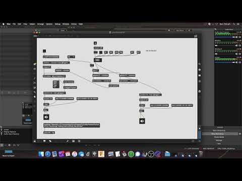
And here’s a qualitative version using the @tutschku method (5 samples played back-to-back).

Also, after some frustrating fucking around, I managed to setup OBS in my studio, so no more iPhone filming of my monitor…

As the results above demonstrate, the matching is better overall with the SP vs the DPA. Although I don’t show it in the video, even more so if I play the original and the single nearest match.

So definitely the way to go, going forward.

A bit of a bump here, although on a different course of discussion.

When I first made this thread, I wasn’t sure what approach was best to take with what I wanted to do (use small windows to predict bigger windows, to then use as matching criteria), but now I think I have a better handle on it.

Rather, I had a better handle on it.

My work at the moment has been trying to build a big enough fluid.kdtree~ such that a tiny (256) analysis window could be matched to the nearest longer (4410) analysis window, to then combine those two together to find the nearest match, but faster.

I knew a classifier wasn’t what I was after as I was going to have hundreds/thousands of individual hits which may or may not repeat or may or may not be similar. I wanted to have a large pool of “most of the sounds I can make with my snare”.

At the last geekout, as @tremblap was explaining why my regressor wasn’t converging we ended up on a tangent (prompted by @tedmoore’s questions) which brought me back to thinking about using a regressor for this purpose.

So I’ve been thinking about this a bit, but I’m kind of confused as to what numbers I should have on each end.

So for the input, I want to have enough descriptors/stats to have a well defined and differentiated space, as the primary features. And at the output I would then want to have (potentially) musically meaningful descriptors/stats which would then be used to query a fluid.kdtree~. In reality I would probably still want to take info from both since the 256 would be “real” and the 4410 would be “predicted” (with some error). So I can kind of wrap my head around this a bit. I guess there may be an asymmetry to things as the regressor (as far as I understand) doesn’t care about the types of data on each end. So I could potentially have a very small/tight set of descriptors/stats going in, and a much broader set of descriptors coming out.

So that asymmetry is a bit of a headfuck in terms of it being loads of variables to try/test with fragility at each possible test.

But where I have a more concrete question is about the nature of the numbers that will be interpolated. Say I have a descriptor space with loudness/pitch/centroid, and then interpolate between points. I would imagine it wouldn’t be perfect, but I could see a regressor “connecting the dots” in a way that’s probably useful and realistic. But if I have a bunch of MFCCs, or even worse, MFCCs/stats that have been UMAP’d, will the interpolation between these points potentially yield anything “real”? As in, if I have more abstract features on the output side of the regressor training, will that lead to useless data when interpolating between points?

A bit of a bump here as I’ve been playing with this with the latest update. It’s profoundly easier to try different descriptor/stats combinations now.

As a reminder this is trying to differentiate between subtly different hits on the snare (e.g. snare center vs snare edge).

I’ve learned a couple things off the bat. spectral shape stuff doesn’t seem to help here at all, and loudness, although often descriptive, isn’t ideal for (timbre) classification as it isn’t distinctive enough. So far I’ve gotten the best results just using straight MFCCs ((partially)loudness-weighted), but even with the simplicity of the ‘newschool’ stuff, I spent over an hour today manually changing settings/descriptors/stats, then running a test example, and then going again.

This is an issue I had before, but process of changing the analysis parameters in the ‘oldschool’ way meant that, at best, I could test one new processing change variation in about an hour’s worth of coding. So it was all slow.

So I basically have 7 types of hits, for which I have training and example data (which I know, and can label) (e.g. center, edge, rim tip, rim shoulder, etc…). I do most of my testing on center/edge since those are the closest to each other and, as such, are the most problematic ones.

I’m wondering what would be the best way to go about to figure out what recipe/settings provide the best results, given that I know what the training data is, and what the corresponding examples are too. Max is pretty shitty for this kind of iterative/procedural stuff, so I was thinking either something like @jamesbradbury 's ftis, or I remember @tedmoore ages ago spelunking similar things in SC. My thinking is something where I can point it to example audio, labels for the training data, then labeled testing examples, and be able to find out that “these settings and descriptors/stats give the most accurate results” without having to manually tweak and hunt for them.

Where things get a bit sticky here is that, so far, most of the improvements I’ve been seeing have been coming from tweaking specific MFCC settings. Like amount of coeffs, zero padding or not, min/max freq range, and then the obvious stuff like stats/derivs. So it’s not as straight forward as “just analyze everything”, because there’s even more permutations involved when starting to change those settings too.

I was also, parallel-y thinking that PCA/variance stuff may be useful here. This is perhaps a naive assumption, but I would imagine that whichever components best describe the variance would presumably also be best for differentiating between examples for classification.

///////////////////////////////////////////////////////////////////////////////////////////

So this is partly a philosophical question which I’ve pointed at many times before where much of (from my experience at least) interfacing with ML is arbitrarily picking numbers that the computer will then tell me are no good, before sending me off to come back with better numbers.

The second part is more practical in terms of if there’s something (semi)pre-baked in ftis/SC that does this sort of auto meta-params-type thing.