Biasing a query

So jumping on the discussion from the LPT thread and the concept from the hybrid synthesis thread I got to thinking about how to bias a query in the newschool ML context.

For example, I want to create a multi-stage analysis similar to the LPT and hybrid approach, but a bit simpler this time. An ‘initial’ stage, and ‘the rest’. I then want to do the apples-to-orange-shaped-apples thing and match incoming onset descriptors-based analysis to find a sample from the corpus. So far so good. But what I’m thinking will be useful to do now, is have a parameter that lets me bias the querying/matching towards being more accurate in the short term vs being more accurate in the long term. Or more specifically, weighing the initial time window more, or the full sample more.

In the context of entrymatcher this would be a matter of adjusting the matching criteria by increasing/decreasing the distance for each of the associated descriptors/statistics. But with the ML stuff, it seems to me (with my limited/poor understanding at least), that the paradigm is “give me the closest n-amount of matches”, and that’s basically it. No way to bias that query (other than generic normalization/standardization stuff).

I guess I could do some of the logical database subset stuff, but that seems like it would only offer binary decision making (including or excluding either time frame).

Is there a way to do this in the newschool stuff? Or is there another solution to a similar problem/intention?

So I went ahead and created a patch that does some of what we talked about in the last chat and made a quick video demo-ing it.

So I’ve analyzed a mix of a bunch of different samples for 4 descriptors with some statistics each, and then analyzed three time scales from the file.

The descriptors/stats are:

loudness_mean
loudness_derivative
loudness_deviation
centroid_mean
centroid_derivative
centroid_deviation
flatness_mean
flatness_derivative
flatness_deviation
rolloff_max
rolloff_derivative
rolloff_deviation

And the time series analyzed are 0-512samples, 0-4410samples, and the entire file.

I chose these as they more closely correspond with my “real-time” analysis window of 512 samples (so I can do like-for-like matching there), and for the Kaizo Snare performance I matched against the first 100ms of each file, and that provided musically useful results.

The results for each matching window is quite different, not surprisingly. I think given the material I like the 512 and 4410 options the most. The 512 gives the most range and surprise as it’s matching the initial 11ms very well, and the rest is a “surprise”. The whole file matching is dogshit, particularly with these samples, as there’s so much fading out during the file that you don’t get anything useful here.

For the variable part of the video I’m using the % matcher in entrymatcher here and crossfading between putting all the weight on the 512 query, or the 4410 query.

So based on this, I think that it would indeed be useful to be able to bias a query between multiple versions of the same n-dimensional space. Because everything is in the same scaling/dimensions/space, nothing gets fucked around like what would happen when trying to bias things towards “caring more about loudness” or “caring more about spectral shape”.

Musically, this makes a lot of sense to me, to be able to nudge a query, or match in a direction that musically grounded, as opposed to selecting/massaging algorithms based on data science stuff.

I don’t really know what this would mean in practice, however. Simply exposing multipliers pre-matching would add some usefulness, like with @danieleghisi mentioned here, though things get complicated really quickly once you have a lot of dimensions and/or data scaling/sanitizing.

I’m going to try to move my querying/matching setup into the ML world (gonna have a jitsi geekout with @jamesbradbury tomorrow), and in the lead up to that I’ve been trying to think of other use cases that I need to satisfy.

Beyond biasing a query, being able to single out individual parameters would still be incredibly useful. I’m specifically thinking of metadata-esque stuff like overall duration, or time centroid, or amount of onsets within a file etc… Things that wouldn’t really be useful to use in a ML context, but would still be incredibly useful in terms of nudging along queries in a certain direction.

I remember seeing some database-esque logical/boolean queries, but I think that was primarily for creating subsets, not for doing individual queries.

With the tools as they stand (or how they plan on standing for the bits that are still in motion), is there a solution or workflow for queries like this?

A naive way for me to conceive it would be where you would ask for the n-nearest neighbors && timeCentroid > 3000.0 or something like that.

Found and played with the 7-making-subsets-of-datasets.maxpat example and this looks like it would kind of do what I want.

I don’t really understand the syntax (or intended use case actually).

Say I have a fluid.dataset~ that has 5000 points (rows) with 300 features (columns), and I want to filter and create a subset of those (something like filter 0 > 0.128). Meaning, I want to keep the amount of columns in tact.

My intended use case here would be to create a subset based on some metadata/criteria which I would then query/match against. In this case I want all the actual features to stay in tact, so I can query them. I don’t want to filter out just a single columns worth of stuff.

I don’t understand what addcolumn (or addrange) are supposed to do. I played with the messages a bit, but none of the examples show the dataset retaining the amount of columns.

The process also isn’t terribly fast. Even with just 100 points like in the example, it takes around 0.5ms to transform a dataset into another one. If queries are chained together, that can start adding up.

Granted this process wouldn’t be happening per grain/query, but it may need to happen often enough to be fluid (say if I’m modulating the filter criteria by an envelope follower or something where the louder I’m playing, the longer the samples I’m playing back are etc…).

Ok, I setup a speed test with a “real world” amount of data (10k points, 300 columns) and I get around 29-32ms per dump of the process.

This is, perhaps, not the way to go about doing what I want to do, but given the current tools I don’t know how else to go about doing something like this. (as in, I don’t want or need a new dataset, I just want to filter through the dataset as part of the query itself)


----------begin_max5_patcher----------
2129.3oc2as0jiiZE9Y2+Jnbk7RhWUbQWyCo176XpsbgrvtYWYIEITO8Las6
u8.HjLxMxVtaod1J9AeADbNmON2.N92eZy1zxWYMaA+KvW.a176OsYitIUCa
L+dy1yzWOjSazO11B1WKS+0s655RvdUnaV.RAo8sV1JxYBw2pXcy71TZwos6
LeB9EyiwyzCUNc+TX+PKZOyKjCVSLzkF6lRcqXSqUTwgm4Em1WyNH5HjOIzC
tCDm34CseEtCfgwdnj.DjfBi8iiB7SjMh8ffeQMc+wSOoda2GCE9dN3TcYaE
3m+dt74a3emAPPr+j.iBTbBH9DmHB9QQDLLwKPJnnPuPaDAS1AP9IJzZoAg1
uyADHbdJCxO4EB2P.7Af.xzP.JwWAAnHeOrMDfh1A7i9PHvw7RIabyU2IU4I
CZEUzZ5YlfUumUPSy0iFdK6gik0moZoK7Q0GBwZKD+HnWh0q3XoIBBA+PnQZ
qPTVb60cWHAF+tQhwxM5FxcDVIaj3PoW.qWDrTf80hs+msXCWew13PzOnWB+
.x4Dl6UfCUsB9YV8jPfzLgZYierrPTHEX8v+O0bZ912hNH+Gv5GYMyJmt51T
K320N.G6EXqO.kQEBCtXFXOCRIrCcLvijd7b1Kr5Ftb8+BarYKspxp4MVCQg
o+Zodhh2MzDunqIzPS0rW38iOXnUZsTNDRgnstC8dMrGlTSSYFqtnkqmotFk
qtFVRuNpP8lJ5gtAqVt669BxDf0hOJVavfR57PRhtfFREkS4kG9MVlkhpbYu
hUvKppYMrBAUXX9gtyXGos4h8iViPRzO.EGNf+td5iFF14T4TQZy1S07rxBE
KMZgQ0bOwkQF5jz.aQS+DEzJGCVpVJQoI5rQJxsMozZ05lwFF22onrLebWCi
KmcTX5thWTbElJJqltyZ9omuwXSKkcd9Vystml8sEc8tWphH12PeYLZKn44F
a+wS+qzBtLNDSY7qEW3Pmc9wdt4PcYd9H4sqmWbzSlTk+.6q7LwyZB4YsdKe
bdUuJ01gU4L9IViXbaB5olwszH9VGna0TapwjdufctJWJEie.owBuQz7b4Wa
LOXuhlM.bI0YaSbaGoiZ+JGpcNvFreux+mc6tBB3vMHzpGG97HZ++nHh1hNn
+8AcesahxymYEcPpLwLV8Kzb.u.btAva.0rpxZAKCHwC1HFuHi8pkeGSvEiK
n2I9LJfy3fNofQ3ysC5d6fNuIr76.3QWQn65eapTUgZusQw50lNOuv9v0qOp
JCjeP4X+lP63f4OF1R9wisHn1JHH7yFb+IoGsUCX8mDXwqNvZbq3qcqPv5sa
9Ihqqnqffefpq9w+esmfvejPaj97.VUGAZ44A0KsfmnIgG3rfmo8+YNwi6G8
WwefFYBnM.YBdx4BPKxLY.HSFvjafyj.v+0AHiWdfryx7QwQpB0L.4MAOWYP
cY6I47hoR5Typp9cipMks0G5wLCz.Fy1x7rE7hgst8kAuff4Zb7n7PzL4A7J
xCgyjGjwXAnUhGBlIODth3f+L4AzJxCjGXsXs3A7L4Axj7fow9CeYqZK0Y66
N9f8Tgnlm1J5LisOMoGZaty6XTNkWlRyuZGrt1q7SWDgk4XAaX4.QMsnQcX0
28t.be.oKzcfDf6tmi.8Gwv03RONl2xy7xnBZCS7mfF94pbVPSaZyPzqok9t
DolBFPwOvkiQtKLPjIpGYejmApjgBweHT4Lqogdh8FXIq8b0zWOhSoM4cbtu
2PZgHOhszFot0GzOj64fj7Ybf+q848K.bPJfOo3qtNuYb6d3ERqF4qSfGQPd
witcOj5BsBWEs5C4LZ8ioVGgVH05.0dWbdMVjnUQXUmmuXG3HOWpuJC38uAP
ODNdGflkcnLu8bA.K43KN66c9obF51QnJX7gx1tDj8eLbDtL3n4hwbq1zchF
gqYHh+aKq9a+4GLxPHZYrgLfg6hD.gWi3k47Fww1hBV9jXf5Qb65HY6h3qzT
aDNCQDDuFR8KrWqpA+siXv+Pc+FHv+T9CD3maNPyo0p6ua3vrla3xvkwdnuN
Q5xQBuNK5osGOxp6yNppTFaPJ6zyUM2rfQFLBlLxJBtL0OjIXh6piH1eMvjJ
F62FgHy8VzsDe21Cj2q8fyDDgqhAQSUsTjOphkzoN72ylEV3DFBVF2BFk.mw
XQQQqUISgTdbAKPYSsLUMUWhjtpjNDF+4sCJ0u+n6eZQSzzYEifBf+EY6SjE
JOytZlyoMvD6dRyMiOexNQ+5yew..u8bWf1G7x8O.r2fwykPgyfNQvEhPn6P
Hj+BPH0NKuqHsDDRMG36PGb7BQn6AcDzBPnHzLftEgPyR8dInjdRt6pDYAnT
vmD14SlCgVBeCphN9tJd9jkhR3OCJQ9rTwwywMTxRPn3YPnfkhP2Uc.tTTBO
GUbzGkRyxXZQVlvygR9KfLglilGZIBLgly5DFuDTZN4ofWh0Ij+LnD4s4Ozk
x2UE6rhHWUjyWUfyus3lmtvlutnl02oVWEcdUZlC2tkLy5vgRatuVgGi.zCG
XEhCk4cb0W.Pu3cp2HIXTn5aQvjXnuTwzpHvUokqGyddgRhY8iEty5M6Qjdx
hFHSul2fdA8f4NypUsjottXU2dVx8ZoGd0p6HA1pLIbKxiDVeLI.mn3ARDV+
OgB5gi7CPF1ewXqQarwMi8dP0i777AAx9JT62dz1S0zLNa3DDLxOZX0NT9JZ
myugrKGb8vv8CKJNVhb6b9s2Nr9QgSfnDsVEwnUo9lrIzUiRtcVSgiGYU8yU
0kpZtoud58HC2tKsUTNHnlkhK2hq6kuwVGyaUztPkmg1kdMyWpVAw5uIkYRx
6VypyIyD+8Ed5Od5+AHvtypD
-----------end_max5_patcher-----------

you actually do every time you change the query parameters. But I don’t see in your patch what you are trying to do… you’re making a 300 dim 10000 entry dataset and you want to get a subset? Why do you time the dump which has an overhead? I have here 30ms for the first query, then 18ms. If I keep all the columns (addrange 0 300) it gets to 77ms which I presume is the overhead of copying more, although @weefuzzy and @groma will be able to confirm…

In my intended use case I’ve got a descriptor space with 10k samples (or however many), each with 300 descriptors (vanilla descriptors, stats, mfccs, stats of mfccs etc…).

I would like to use one column of that (timecentroid for the sake of simplicity here), and bias a query based on that single number. As in, return me the nearest match (along all the dimensions of the descriptors) that has a time centroid above a certain value. Or find me the nearest match where the loudness is below a certain value (this gets weirder).

But the overall idea is something along these lines. Where some columns in the thin flat buffer correspond to data that I’d like to use to query against in a more direct way.

That’s how addrange works! I kept trying stuff and didn’t couldn’t get the default example to return every column it started with. (I could have sworn I tried addrange 0 4). What happens when addrange is backwards, like in the example? (addrange 2 1)

its not backward, it is like all our other range interface: start and num
0 300: start at 0 and gimme 300
2 1: start at 2 and gimme 1

===
In your case, if you’re going to bias a query on a subset, then query in RT, you make the subset, you then make a kdtree of that subset, and query that kdtree. the query should be faster than on the real dataset since you have less values. what is even better is to query only what you care about, so you could dismiss the columns you don’t care about and make a smaller subset in that dimension too (nb of dims)

Right. It’s just visually confusing because there is no associated message that goes with them, and addrange 0 5 returns the data I want, but for visually confusing reasons (as in, it looks like it goes from 0 to 5, inclusively). I’ve mentioned this already, but this <dataset> <dataset> <number> <number> syntax is a lot more confusing overall.

I tried to make a dataset that would have around the amount of numbers I’d be dealing with in a realworld context. I can easily get up to 10k samples/grains/bits and 300 descriptors/stats is about par for the course these days. Granted my realworld numbers may be slightly smaller, but I wanted to test it with numbers greater than 100 entries and 5 features.

I perhaps wouldn’t need all the columns for each query type, specifically if each column corresponds with a different time series and I’m choosing between the initial 256samples, or the initial 4410 samples etc…, but if I have a single value in that column that could potentially update on every query, I’d have to do this process per query.

edit:
To further clarify. It wouldn’t always need to update ‘per query’, but if I’m doing the thing you (@tremblap) suggested ages ago, where I have a slower envelope follower going, and us that output of that weighted against the current analysis frame to decide how “long” (or higher ‘timeness’) a sample to play back, that means I would need to update things per query.

Kind of an old bump here, but I think this thread is the most relevant to this discussion/idea.

After getting some ok results using a regressor to use a short analysis window to predict a longer one I was wondering how to best implement this in a patch.

Ideally I would take the realtime audio input (analysis window of 256 samples) and compare this to the corresponding window in the corpus,

and also

use the regressor on the realtime input to predict a longer window and then use that longer window to query the longer window in the corpus… with less weight.

I was thinking that a “lofi” solution to this would be to concatenate the realtime input descriptors/stats (8d) with the predicted/regressed one (also 8d) into a 16d point which would get compared to a concatenated 16d for the corpus (8d of the first 256 samples, and 8d of the first 4410 samples).

But this would give me a 50/50 weighting between the “real” data, and the predicted one.

So I was wondering if I could just double up on the initial 8d by duplicating them so each point would have:

8d of first 256samples
8d of first 256samples (a literal duplicate)
8d of predicted 4410samples

and that would be used to query:

8d of first 256samples (of corpus)
8d of first 256samples (of corpus, a literal duplicate)
8d of first 4410samples (of corpus)

I was thinking I could also achieve similar results by scaling the 8d of the 4410 windows down, but there aren’t simple ways to transform a buffer this way on the fly (as far as I know). I was thinking I could perhaps do something weird like creating a fit using [fluid.normalize~ @min 0. @max 0.5] and then use that to transformpoint the corresponding realtime input, but not sure if that would behave as I would expect.

Any thoughts on this kind of “lofi” weighting?

I think that at that point, you might overload the fluid.normalise object with loading your own scaling per dimension. To check the format, dump it first in a dict. each value of bias is added and each value of scale is multiplied.

Hmm, you lost me there.

What I was thinking was that as part of the normal processing chain pre-regressor (robustscale->PCA->UMAP->normalize) I would set @min 0.5 @max 0.5 such that the whole of this dataset would be scaled down, with the corresponding realtime version being the same.

I guess I could just keep things 0.->1. for the regression step but then normalize the output afterwards? Does transformpoint allow you to apply separate @min @max attributes to the output or does it literally only apply what has been fit?

And/or

Is it bad to send fluid.normalize~ @min 0. @max 0.5 data into fluid.mlpregressor~ @activation 1?

no. but you want to bias the query, so you might as well bias the relative weight of each dimension.

check this example. it not about fitting a standardizer but using it as a scaler - subversion is fun :slight_smile:

standardize-hack.maxpat (15.7 KB)

I was planning on applying this transformation to only the regressed/predicted dimensions, and leaving the analyzed ones intact.

So effectively doing:

8d of first 256samples
8d of predicted 4410samples (scaled down)

Would the fact that it’s standardized (vs normalized) really matter here if it’s just changing the min/max?

And correspondingly I suppose this would have to be with a different @activation in fluid.mlpregressor~.

no problem - use my hacked standardiser (you will notice it is not ‘fitted’ and independant) with transformpoint for your query… but using that in anything else than a kdtree is definitely not going to work - this is a way to squew the euclidian distances…

it is like changing the range manually for each dimension. i use standardize because I know how it works under the hood.

Returning to this today and hit a bit of a snag as the regression I’m doing before this has no interest in converging on standardized/robustscaled data.

I know the loss amount doesn’t mean anything specific (is it in relation to network size or something concrete at least?*).

If I take my “real” 8d of perceptual descriptor (loudness/centroid/flatness/pitch) and normalize them, I get a loss of 0.086 with fluid.mlpregressor~, which to me, seems “good”. If I apply robust scaling instead (and switch to @activation 3) the best results I get with the same network settings were around 6.25. I also tried with @activation 0 and that wasn’t any better. I guess having the outliers pushed to the edges past the standard deviations doesn’t make the regressor happy.

SO

I can run the regressor on normalized data, then take the normalized data and robust scale it to prep it for biasing, but that seems weird/wasteful. But would that be in line with what you’re suggesting?

*I got the best results so far with @hiddenlayers 6 4 2 4 6 with 8d of data on either side, which seems odd to me as that’s a huge network for such a low amount of dimensions. Is the loss value proportional to the amount of points (entries * dimensions) in the dataset, or the network, or a combination of both?

The tl;dr here is that in general you’re better off returning to the data itself if there are problems converging. First things to try might involve seeing if things work with a lower-dimensioned slice of the same data, and / or a subset of the training examples. Moreover, it’s pretty important to hold some data back from training to use as a test set, because the mere fact of convergence isn’t enough to be sure that a network will generalise to doing something sensible with points it hasn’t seen before.

It does mean something, but the number on its own is not sufficient to diagnose whether or not a network is converging. What the number represents is the mean squared output error for that round of training, i.e. the sum of (predictions - truth)2 divided by the number of points. So the scale is a function of the overall range of your output dimensions and the number of training points. The power of two means that the number will get rapidly ‘worse’ for errors. One thing to note here is that this is essentially a distance measure, so if your output points don’t have roughly uniform ranges, convergence will probably be slower (because errors in output features with a large range will have disproportionate influence on the network’s adaptation).

By and large, though, the loss is useful as a relative measure. First, watching how it changes over repeated bouts of training can provide some indication of whether the network is converging at all: stick a multislider on it in history mode, turn down the number of iterations and hit it repeatedly. You want to see the loss decreasing, ideally exponentially but it may well plateau for a bit and start going down again. Going up is generally bad: if it’s dancing around, then the learning rate is probably too high.

However, tinkering with the network shape and learning controls should be secondary to reassuring yourself that there’s a tractable problem there in the first place, which is where trying simpler problems is valuable. By trying single dimensions at a time, for instance, you can see whether some feature in particular might be causing problems (because there’s no structure in the mapping to be learnt, perhaps).

By holding out some data to test with, you can better understand what the network seems to have actually learned. Fire some test points in, and look at individual dimensions to see whether the learned mapping is all over the place, or seems to break down at particular points.

1 Like

That’s useful information. Thankfully I’m regressing on “natural descriptors”, so I can feed it points and see if what comes out seems reasonable (re: loudness, centroid, etc…) by looking at the actual numbers.

How does one approach “checking” if you’re feeding it more abstract data (mfccs->pca->umap->norm) where the numbers are far beyond gibberish. I suppose I could check to see if it’s doing what it’s meant to be doing, but in my case that “doing” is “ever so slightly improve nearest match in a corpus”. So that’s a bit intangible in terms of how effective the various results/mapping are.

I’ve been doing that trick of looking at a multislider, and having a low maxiter so I can loop over results and check, but surely there’s a difference of seeing the number go down a bit and plateau at 6.25 and seeing it go down a bit and plateau at 0.086.

This is a bit tangential as I imagine the answer is close to “this is how it’s done in the literature”, but if the loss is proportional to a fixed number, it would be way more useful to have a number that is normalized to that (e.g. “3% loss”) instead of a super abstract number where “lower is better”. The trajectory could still be observed, and lower would still be better, but it could at least be comparable to something else.

///////////////////////////////////////////////////////////////////////////

Slightly more on topic is a bit of a brain fuck as it now seems like my corpus querying prefers having robust scaled inputs/corpora whereas the regressor I plan on implementing prefers normalized data.

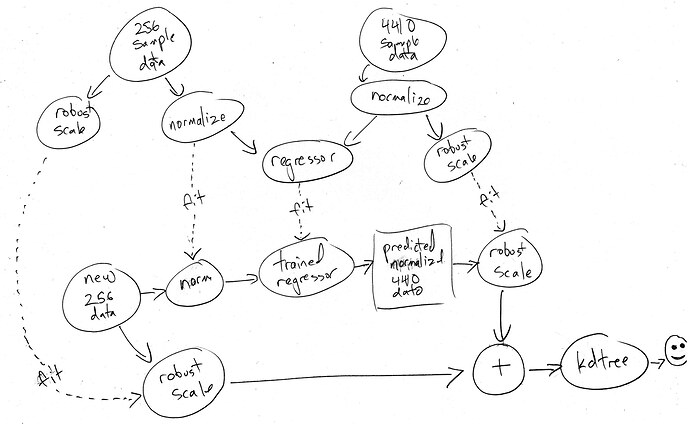
I think this is how I’d want to process it?

I suppose the results of [data->norm->IQR] and [data->IQR] are the same, so the left side could mirror the right side in terms of [data->norm->IQR] for simplicity, but it was useful to draw it out this way.

I may also shape the robust scale on the output of the [predicted 4410] based on @tremblap’s suggestion so it’s not a straight concatenation at the + step at the end.

A general comment is that interpretability of machine learning pipelines, especially stuff like deeper networks, is an unsolved problem, although there’s a lot of active work. In general it can be easier when the processes are invertible, so at least one can get back to firmer ground, but that’s not always possible. I do note that the the reference implementation of UMAP now has an inverse transform (with many caveats) so it might be helpful if we look at implementing that some time. Similarly, one can (kind of) invert MFCCs back to a (blurry) mel spectrum in principle, which could be useful.

Meanwhile though, back to the topic.

If the 6.25 is from robust scaling and the 0.086 is from normalizng then you don’t know how much difference that hints at without knowing the range of the output points in both cases. For normalized, this is obvious. For robust scaled, you’ll need to look because it depends: like, if it turns out that some dimensions have outliers with values in the hundreds, then this would suggest that the actual convergence isn’t so different.

As for the loss number, I’m going to say again that it’s just not that useful by itself, and when only applied to the training set. You really need to keep some data back (and we need to make it simpler to (a) do that and (b) produce a error measure for a test set). As for whether there are measures out there that would make a more easily interpreted number: yes and no, especially for regressors . We could look at implementing an R2 score but there are some health warnings about its interpretation.

In any case, if you’re having problems getting a manageable network that converges reliably, I still think the thing to do is go back to the data and try with different subsets so that you can look at smaller problems in isolation. Tweaking the network hyperparameters doesn’t get you very far on its own.

I’m not up to speed enough with what you’re trying to do to pronounce much about your workflow, although I don’t quite follow why you’d be summing your input and predicted points before the tree lookup.

1 Like

That makes sense. I had forgotten that the scale of robust scaling is unknown, by definition.

I guess the fundamental thing is that I have no idea if the network is converging reliably. Sometimes the number goes down, sometimes it doesn’t. Sometimes the number is small, sometimes it’s not.

With my “dumber” testing more recently, it’s a bit easier to run tests as the pipeline is pretty straight forward (no pca/umap), but it’s still black boxes all the way down.

Summing isn’t what I’ll actually be doing here, that was just for the diagram. My plan/intention is to concatenate the real 8d with the predicted 8d, then feed that into a KDtree that has real versions of all 16d (via offline analysis). As per discussion above with @tremblap I will likely scale down the predicted 8d (and the corresponding offline 4410 analysis) so they are weighed less in the distance matching.