Dimensionality reduction (mixing the rational and irrational)

[rodrigo.constanzo]

As part of my attempt to move some of what I’ve been doing into ML land (and after having a fruitful geek out with @jamesbradbury) I wanted to try to use dimensionality reduction in a way that still “made sense”.

That is, my understanding so far is that once you go into dimensionality reduction land, you give up the ability to have numbers that relate to real-world units or have “meaning”.

I remember @tremblap mentioning he wanted a better “timbral” descriptor for his LPT idea, and wanted to have a way to have 12 MFCCs reduced down to a single number which better represents the overall timbre than centroid+stats. MFCCs are intrinsically weird numbers though, which I’m sure complicates this a lot.

So I thought about trying to reduce a bunch of my metadata-esque “timeness” units. Mainly things like duration and time centroid, and potentially things like the derivative of loudness (and perhaps at several time scales). I had initially posted some thoughts about this here, but that was before we had the dimensionality reduction tools.

My hypothesis (and goal) is to have a single value that corresponds with how “long” a file sounds, by weighing the actual duration, along with the time centroid and derivative of loudness. That’s the hope at least.

/////////////////////////////////////////////////////////////////////////////////////////////////////////////

So I’ve whipped up a test patch, partly for me to make sense of this workflow, but also to see what kind of results I would get.

It creates a fluid.dataset~ filled with units that correspond with milliseconds (0-5000ms) as well as one that corresponds with milliseconds along with some derivative-like units (-2.0 to 2.0).

I purposefully didn’t standardize/normalize the data before fluid.mds~-ing it, since I wanted to keep some differentiation in scale between the different numbers (perhaps a big mistake). I kind of hoped (and falsely intuited) that the numbers that came out would be roughly in the same range/domain as what goes in.

That is most definitely not the case…

Normalizing the data afterwards obviously doesn’t help either.

I tried fluid.standardize~-ing the data pre-fluid.mds~, but I’m getting nans and (end) as the values everywhere, and I don’t know why (separate concern/issue).

So I wanted to post the code, but also ask about this general approach, of using dimensionality reduction to create macro/meta-descriptors which fuse together related data, which is then queried/matched in a contextual way. (As opposed to shoving all the random numbers in a black box and hoping what you want comes out (which I’m not opposed to I guess ))

----------begin_max5_patcher----------
3536.3oc6c88jihaD94Y9qf3mRpLGAIgDPd5RkKUkpR1mRkm15povFrG1ECN
7icm8t51+1iPBvBavVXK4AOGmqyiWIvp6O0cqVBoO+qO9vhkouFluv3uZ7Qi
Gd3We7gGXEUUvC0+6GVr0+0Uw94rKawpzsaCSJV7DuthvWKXkmjls0ON5WBC
L1Fj2T8trvb5U6WDkl7bbTR3pzxD1M.quh0oIEI9aCYeI+yv3uDVDsxu49iB
Xkmt7S+fMXgvsr1eE6V.0kkTtMJINrH+fBSKKZJ0R31yoBJSJrLaJdmewpWh
R17bV3pBNh..Ntz5Mbwfp+.Hr+.IlVF+b0M8aO9X0aOckPWl+WEwL4QDqaNh
3BrD.DOKsgGA9E9iFPPd2b.ABwlNXUgHaCyy82DdDhDTtcWSgbws3a6B4Rvh
EF+bOPAZQepMrW0FbBW.KKTkJgrvlt.wWHZgdLsEdgZaPzpByuDE90d5JgvE
iua6Dtv1tDlKLFxzFB5Bk4jvuREui6fpTk.ZrtrHVPvA6rptPZrP+ru0a2FD
MB0FHgZaCMcf6eQ7.sFoP0BAYTIKz3zVpOMf0JzYDVqvyq1HOGSKOgWDpKJw
SGp853xn.ypvU4gEe2nHhFRi5Eate7vAgik9Iapfj0wo9EChM.2QXRfjvSlF
oxFK7B4Q8K7ruJvYn.WqiJJx7SxWSQi8XSVXP4JZhBiAr52tAn1nb.hqonYi
GhZ2.c0n+hH.cA9MVJxuoV+gDKyNA4ccnfhki9bbZ64+twOR0.CZ6S+f+qzO
3csNNdp0wABrME8avDPEp.0A3PyadWXRfAMlx37H.D0L.hq6vNDNZQk82wzX
qQpuX0nuDKhIDOPmL95F4njFkqbP0JJgaB20LtHba8zxV7A+jW7KJ7Sptjmp
d6eTtJNJHTnj+y+qzmFU033Z9PTR5Wy+bjwG7esmBi1ek+qx33k9q9rw+NLZ
YXlweLIsv3agE+o1q3umlSmBW+8C1sS4yOilqdQX1ygI9KiCESP65bDarIgH
SnXRMtU40QtptnglJRUjFisg+gQOUD.71OUDDCCP7Ih3bUSD4JMYKSh3CnQS
3kMQtZCnsQuVMDeco8ZGYcCri3yAf8NM3tNBl8mM.mD85S08TStLbsywwjfD
dYS0QOSr50zM9zrXfmPcGb7YW0j6BWe6MnfsVRbYmw1xUuj9STS3+aic94Vs
KznFTyVQigCGbHbfXZKheCgY0.RMhPC.EEG9kvrbpNIzdOTMdsPwOHbKUv3m
RYeQtO0VDcHmLwufGVjE9knl6G2VpeFUOJnJQYFOL6qjF7n5qIMHLKoLh8Mw
Kj1gVKRrttpvy46pC3x5gapdOxvGPGXwlzCcRir+IFZuGMn1FahSW84v.g3N
z9OZNJQIh8ycpNHbseYbwyhAsAPydquYLgdqrcLl+V0BJzpAaxhBRSpDhNcE
UE2zbz7Uw7U5PTYXWQh+tdtYpAGEWFnxbpRVluzOqpmpNHLroxhzz3tU0dew
gqKpqdWTRxAnXQ5tgqLKZyKm3dWlRqb6o9tY0j+bYBu1moFEEOm6+ktncgeb
bsCd2u9W8Sh1RCpUM4T9ftsUxGH5k7UYowwczWdMeomZBnF4qB+ZTPwKrFRz
Xfd4Q6ZLhVz1KGDsILunaYE9ax6VRdw23ftPQkKqchelNX7tXpVz8BntGQ4E
4uPS9q9BaLzDAf8OP.QmZwnkcJ+TQM6F4LekebHEBL.lUuioi8JdcCGbbvY4
bbTRR2JNNR4vSyCvV6HXcXy5I80N3wCMCfTGyQ8vyeoJajygI747NHv3LHv.
uZfAg4gIu03RleRP5VN3bRrQLypAWFMMfL.OFl3Rt0Hi5bn7TuCkq28u+DzR
8VMM3xcs6T6JupdfYp3MArtX2o1mdkBcmbb53NArtGcmPp2poAWtucmr0Fv7
NvcBnduIB9cf2j5sYZfk6ZmIj1vk2A9R1p2WBit+8kvp2loAVtq8kHZCWlPS
Z5R8kbTuujM392WRCyz198vRP3oMb4MyWp7WhpVfzSBIM6Vil+dJHBeIXD5z
XDDZK7j9N7YBoeL5SoQIF.qKKDCdXmIf0EGA1huQv3ONcKOu62PvXj5iACq2
fj204yngIT1fK20AgwXsALuCxnAaogGrhy6.2IMrbmM3x8s6DTa.y6.2IaM7
XUv2+dS1ZXFB32ANS1N5BWzquDSLuLODxv4ucwo2VmvuMOK2126HBMa3SwsG
ASzRBBeUXyEoD7gK5KF.AFNSMvfHfkLc517sBpJQf86nnps21.6SDl.Ey1ov
8AM4okYqZLLZ1zBFcEtfv7hnj1MX0G2usOLj0zczRAQRonZJYFtZRJpdfyxg
Ed5DK7FCV3nKr.IoTT83V0FVz7kKGVPzkTHqYgNsJFCPf0jP3JoP3nQfvYL.
ARW8FxhD.cBEPYMJZBroGovVVo.oQoP5vUZTFrGioostDBYcPrc0ITHqChsN
GJ0dTCkpKo.KKTnSYvZLHAPWRgzihoy.VXoSpPmCniQioGApKoP5XV5L3MVV
WDrV8QjMlEQmRgzyDRixfrgM0YTShz9G5bDDrrPwwWWZV.+.cgeakLxvRl8a
qj0iaeqnQdiEM3vhlyaqn0SBdshl6aqngFVxPusRVOSRoUzfuwhFXXQC71JZ
8LM2VQyp2Un7QwCE5hpC9Wvy7C43y9EEYQKKK3qbo3obcTGFuMwoK8iO3Dz0
2Y06w8B2aFSfQbTy4JmfALFx3VyDXDW0vDX0TW2cBQfQ7TzY.uVquO3ALGjh
3D.tVOAnArZpt5JoxHGa0PkQDNKE1OEfUeNZzCaI7gJl+3mDH0QICdoH58Ax
MH5mKD.ybgvLWHLyEBybgvaEWH7CPSC3zkJDNjaHmYBgYlPXJyDBWk6j1IBg
6RuoYdP32o7fv03KoeVP39zWZlDD9cKIHfmvbfv8IA8LyABybfvLGHLyAByb
fvaiuzLGHLyABybfvLGHLyABybfvLGHLyABybfvLGHLyABybfvLGHLyABybf
vLGHLyABus6G54cQ9Deu2OcOvBS3S4wD9rwLgOQQS2ig0M+nqMMNZeSgC43L
gZLgN0qSiy+6D4rPOMNW3SiyH+zfu.lFbmvzfGIl.LpwzfaQlH7rxzfyYlBz
uyTfGhlFLxzLCxM4XpqIA+FNIXSuIAGKNMXQtYF.Uorr3LGHLvNa7Jo.AHx0
DOvwmViLffiZH.AHDa5PEeLh+nAvrcADhe3XmdLf..oni9csZWS7CWIoGPcb
JntGm7372m1fZYwhc9YTukhvrm4GTVwdMkbH2Q7G7mcy6prysfQrCFKoQnVE
G5mMbmKyGs6Fdi9G9M0K.QFQ2s8YAAGGSBR3k8SM0bwc8CEN5z.Q+JqhBHA3
aas9CHg0h1leJW59UVaEorDHyQtes8J4xjxsKCyNIgkLrqMTQt1vyq61ttlh
l0HfySMO1esviKUc2RPlKCQbIHqd66Qik3RZ0+93wFfMVKLWh+mM7CB1kRic
YD0RoKiy3G5MB.3Tw1sGl3VPZQ8WkVlTbBeh5H5M+u3d5nC.zO8MgGabc9d8
oWxmxinC8ONJuXcYRRX7fPP0kzuRSTTtKVnpDNgDKyNJsakWuVz5cgge96m2
Vu6dapipiUjAOW06uCGoCUuflVS7YIpo9U5wvOSvyYjCA1lhN4XBKHmEyTP0
imuNhNeP+j70oYa2SaUUDY0QjXkAXjj2jhHdNKBi345k7lfXr9nyqsA4e+JY
tKjhHtqZLn2HADac.AKKWuNLaer.ieL2e6t78mhighJbpbkfpwOw1hsqt.Pj
ITLc.2JqD7sje2BNEklImIBPMlH0YHzGk2Av8SsaLoo6tXiCQGtlU0.0wOoA
K9SXqVpjXWmbvlU6nNGYaYmNqruTaHsEai3Iyk2PRfdUQTsgdGiXdt70H4D0
AvN8vkbV.nIt2JUMBzckzGZykI7zUt3VBICVCbUPKApeF5mtW0QAsDTJ6GnJ
ZIGYZIUzOwdhBmE8rTgNAjwhvSE5DVFqbEzPDYzHrJznwzRCD4xiEjAZAMgh
i+YSG+i.3K2YOUdsBtsLBNQAPjTA2Id8OtB35ZZaI7gbTRTUorCTQC4JiKDQ
UpzYC.IrOottVBctVRGIdHUKCzgoIqkOWxVtctlCha.cQl.hv+A83GeJOwoa
RbplBJK2ndp6ZCyJS7bnsBLFsuUMjmDMjJRNxUlbswJpgNmBoBfCHSFrpHIB
jDgkHpHqRhL1BDUXLPjIqRGUzKguUCScyZH6aUCI0LzfppkNWrA.RGiJA8tQ
nITlvRLoAbssjLYlAUQjVnTCR4ppV5bVHPUjDHPlj2UQvVfDQ0QGOaW9hdc.
i8W0FGvT+GvR+GyP+CyN+GxL+rMhEmjxOXg1Z23Ta8ekzxO+MzeeW.ve0pvj
hUowbo5iFVlz46QeC4AAjpO4X44ZYS6mE9kLnZELY2yyQIUZbXy8Z8jvah2w
xMBsAnt152rLwMf4S0cVYTg5P9WewVpzG0jrsXmaGEV3LS2uJ2QYsgHbUBqV
lHGH1l8I5zZwfZwWYhUmGUR+B1kfpqihiaUHw8cWyJFuXSlePT04Qt8GwgpK
Gz1aWkxtyS89If3uvAraC1baNttvp0lruOc7s0bWPOKfGypBUaUU8IZQfCtK
+jM0+VH3HPn+6xR2kl09iBgIxq85KKRaUz1CsbyFDr+tutdGx0KJdfykv5h0
mQmgimEj8IpNyd35WlkEOHy.+Fb73u83+GDTrc4A
-----------end_max5_patcher-----------

[weefuzzy]

@rodrigo.constanzo

I kind of hoped (and falsely intuited) that the numbers that came out would be roughly in the same range/domain as what goes in.

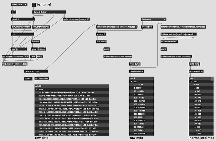
Absolutely not, no. In the case of PCA, the output range will be in terms of standard deviations (so mostly within ±3 for data that’s normal-ish distributed). For MDS I’m not so sure, but you seem to be getting some values at least comensurate with your largest dimension in the screenshot above.

But what do you mean by the ‘range that goes in’ here? In the un-normalized case, you have dimensions of sugnifciantly different ranges, which is going to give unpredictable results. I would definitely normalize / standardize here. (If you think there’s a standardize bug, please do report it)

So I wanted to post the code, but also ask about this general approach, of using dimensionality reduction to create macro/meta-descriptors which fuse together related data, which is then queried/matched in a contextual way.

Yes, that’s a sensible thing to do, although I don’t completey grasp what matching in a contextual way is getting at?

[rodrigo.constanzo]

@weefuzzy

Absolutely not, no. In the case of PCA, the output range will be in terms of standard deviations (so mostly within ±3 for data that’s normal-ish distributed). For MDS I’m not so sure, but you seem to be getting some values at least comensurate with your largest dimension in the screenshot above.

After winding down for the day I thought to try PCA since it’s the “dumber” of the choices, that it might go with what I’m trying to do better.

@weefuzzy

In the un-normalized case, you have dimensions of sugnifciantly different ranges, which is going to give unpredictable results. I would definitely normalize / standardize here.

I wanted to keep a sense of the difference in scales between the (currently random) entries, but I guess that would still be the case if I either standardized/normalized them anyways(?).

@weefuzzy

Yes, that’s a sensible thing to do, although I don’t completey grasp what matching in a contextual way is getting at?

Me neither!

I guess one a simple/pragmatic sense, I could “mix” a bunch of related descriptors together (duration/timecentroid) and then use this single “timeness” metric to bias the query.

So rather than having to chain things together (duration > 1000 and timecentroid > 500), I can just query for timeness > 0.6.

This is likely just me entrymatcher-soaked brain trying to make sense of a knn-y world though.

@weefuzzy

(If you think there’s a standardize bug, please do report it)

I’m nowhere near confident that it’s not a meatspace issue with that, but if I find it, I will do.

[weefuzzy]

@rodrigo.constanzo

After winding down for the day I thought to try PCA since it’s the “dumber” of the choices, that it might go with what I’m trying to do better.

It’s a case of try-it-and-see. PCA can only produce a linear mapping, which constrains the complexity of relationship between spaces its able to represent. Intuitively, the more drastic a reduction one wants, the more likely it is that having a non-linear aspect to the transformation will be helpful, but it really depends. So, yes, try PCA and see if the results correspond to a sensible representation of ‘timeness’ for your purposes.

Also, with PCA it’s a little easier to grasp what the effect of differently scaled input dimensions will be (because the process is linear), i.e. dimenions with larger ranges will bias the reduction in favour of those dimensions. It’s not at all uncommon to do PCA first and then follow with a non-linear reduction when trying to go from lots of input dimensions to very few.

@rodrigo.constanzo

I wanted to keep a sense of the difference in scales between the (currently random) entries,

This is the bit I’m not following. Keep a sense of the difference in scales for the purposes of weighting the dimensions’ relative importance in the reduction?

but I guess that would still be the case if I either standardized/normalized them anyways(?).

No: the normalisaing / standardising is done per dimension, explicitly to remove the difference in ranges. At this point it’s more productive to think about how the input data are distributed

@rodrigo.constanzo

I guess one a simple/pragmatic sense, I could “mix” a bunch of related descriptors together (duration/timecentroid) and then use this single “timeness” metric to bias the query.

In which, yes, this is a perfectly valid approach, but it hinges (per above) on how well the reduced quantity really represents the thing you’re trying to capture. In general, squishing something down to 1D will require a certain amount of experimentation because you’re throwing out a lot of stuff.

@rodrigo.constanzo

This is likely just me entrymatcher -soaked brain trying to make sense of a knn -y world though.

They’re not so different!

[rodrigo.constanzo]

@weefuzzy

It’s a case of try-it-and-see. … It’s not at all uncommon to do PCA first and then follow with a non-linear reduction when trying to go from lots of input dimensions to very few.

I’ll try PCA and see how that fares. I think if I’m just in millisecond land, it would (intuitively) give results that made sense that way. If I include derivatives that would probably crumble without sanitization.

Curious about this PCA->non-linear workflow too. By this do you mean do PCA on something to bring it down to a smaller amount of dimensions and then to do MDS on that lower dimensional version?

@weefuzzy

@rodrigo.constanzo

I wanted to keep a sense of the difference in scales between the (currently random) entries,

This is the bit I’m not following. Keep a sense of the difference in scales for the purposes of weighting the dimensions’ relative importance in the reduction?

but I guess that would still be the case if I either standardized/normalized them anyways(?).

No: the normalisaing / standardising is done per dimension, explicitly to remove the difference in ranges. At this point it’s more productive to think about how the input data are distributed

I’m not really clear on things either, but say I have one file with a duration of 5000 and a time centroid of 2500, and another file with a duration of 400 and a time centroid of 200. By not sanitizing the data, I was hoping to maintain that difference in scale, rather than them having somewhat similar values (?) after sanitization.

More practically, I want the fact that the first sample has bigger values to be present in the ‘timeness’ metric that I can query later on, if, for example, I want to choose samples that are ‘timeness’-ier (yikes!).

@weefuzzy

They’re not so different!

In spirit I guess, but I’m still struggling with my normal use cases where I can find the nearest match for certain fields, and then some other criteria for other fields (ala biasing).

[weefuzzy]

@rodrigo.constanzo

I’ll try PCA and see how that fares. I think if I’m just in millisecond land, it would (intuitively) give results that made sense that way.

Depends what you mean by making sense. The output ‘units’ of the PCA will still be in terms of standard deviations, so won’t bear much resemblence to the millisecond input.

@rodrigo.constanzo

Curious about this PCA->non-linear workflow too. By this do you mean do PCA on something to bring it down to a smaller amount of dimensions and then to do MDS on that lower dimensional version?

Yes. You can think of it as using PCA to make the job of MDS easier by stripping out some redundnacy / correlation in the input. So if you wanted to go from, say, 300 input dimensions to 2, it might be worth PCA-ing down to (say) 50 or something.

@rodrigo.constanzo

I’m not really clear on things either, but say I have one file with a duration of 5000 and a time centroid of 2500, and another file with a duration of 400 and a time centroid of 200. By not sanitizing the data, I was hoping to maintain that difference in scale, rather than them having somewhat similar values (?) after sanitization.

The difference in scale would be preserved with either normalizing or standardising; what’s changed is the weighting between the durations and the centroids. In this imaginary two-item data set, normalising would give you two points [0,0] and [1,1], so definitely not similar values). Standardsing would give you two points [1,1] and [-1,-1]. In both cases, the difference is scale is accounted for (quite drastically)

[rodrigo.constanzo]

@weefuzzy

Depends what you mean by making sense. The output ‘units’ of the PCA will still be in terms of standard deviations, so won’t bear much resemblence to the millisecond input.

Ah right. Yeah, I misunderstood that.

@weefuzzy

Yes. You can think of it as using PCA to make the job of MDS easier by stripping out some redundnacy / correlation in the input. So if you wanted to go from, say, 300 input dimensions to 2, it might be worth PCA-ing down to (say) 50 or something.

This makes sense, and I’ll have a play to see. For the purposes of this example the starting dimensions will probably be more more than 10ish (overall stats like duration and time centroid, then multiple time scales of loudness derivatives and maybe deviations?). So for these kind of “meta-descriptors”, I wouldn’t have such a massive set of dimensions to start off with, but they are likely related to each other in a more linear-esque manner (e.g. time centroid will always be shorter than duration, the ratio of time centroid to duration may(?) correlate with the derivative of loudness, etc…).

@weefuzzy

In this imaginary two-item data set, normalising would give you two points [0,0] and [1,1], so definitely not similar values). Standardsing would give you two points [1,1] and [-1,-1]. In both cases, the difference is scale is accounted for (quite drastically)

So if I understand you correctly, both standardizing and normalizing those examples would happen in a way where the it would be impossible to tell which one of the two was “longer” in terms of realworld milliseconds. the 2500ms would become either a 0 or -1 and the 5000ms would become either a 1 or a 1, and the same would happen for the 400/200 version.

Maybe this kind of approach would be better suited for vanilla number crunching where I take these numbers and feed them into a function with relative weighting taken into consideration, and it spits out a ‘timeness’ value that way(?).

I still want to push further along this dimensionality reduction approach as it’s a useful vector of getting my head around it, and it may very well be a good approach to do this, but it’s a funky bugger!

[weefuzzy]

@rodrigo.constanzo

So if I understand you correctly, both standardizing and normalizing those examples would happen in a way where the it would be impossible to tell which one of the two was “longer” in terms of realworld milliseconds. the 2500ms would become either a 0 or -1 and the 5000ms would become either a 1 or a 1, and the same would happen for the 400/200 version.

On the contrary: in either case the dimensions still exhibit the same ordering after standardising or normalising because all that’s happened at this point is that they’ve been scaled and shifted. So for normalising 5000ms → 1 and 2500ms → 0 because these are the extreme points of the data set (by definition, because it only has two points). If you added a third point of 3500ms this would become 0.4.

However, after doing any kind of dimension reduction, there is indeed no way of determining which file might have been longer to start with

[rodrigo.constanzo]

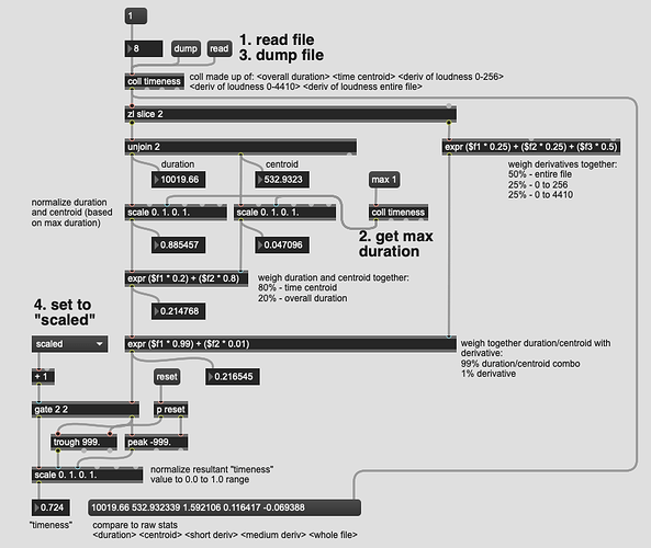
Ok, I took a stab at “manually” creating a timeness metric.

This time I’m using actual values extracted from a larger corpus. I’m taking the overall duration, time centroid, derivative of loudness for samples 0-256, derivative of loudness for samples 0-4410, and derivative of loudness for the whole file.

I started playing with this “intuitively” by trying to weigh different bits of this together, and then trying to merge them.

I started with just the derivatives. I first thought to put the most amount of weight on the first time window, but then thought that it wouldn’t best represent the overall file, so at the moment I’m weighing them like this:
expr ($f1 * 0.25) + ($f2 * 0.25) + ($f3 * 0.5)

I then normalized the duration and time centroid by the maximum duration in this particular corpus. I weigh the normalized centroid with the overall duration, with the centroid itself having the most weight (80%), with my thinking being that that single number probably best represents how long something sounds. I’m weighing it against the overall duration as that would have an impact too. So that gives me:
expr ($f1 * 0.2) + ($f2 * 0.8)

The next bit was a bit tricky as I wanted to take the value I got from mashing the centroid and duration together (which are grounded in units of time) and have those impacted by the derivatives.

For this particular corpus the derivatives (when weighed together as per above) range from -1.051384 to 5.505389. My thinking here is that if the file is going down more than it goes up, which would correspond with a negative/low derivative value, that I would want to bring the overall timeness metric down. And the opposite would be the case for a positive/high derivative.

Since the ranges here vary a bit, I’m only giving a bit of weight to the derivative here with:
expr ($f1 * 0.99) + ($f2 * 0.01)

Finally I take the overall timeness and normalize that back up to 0.0 to 1.0 so for this particular corpus, I now have a ‘timeness’ metric between 0.0 and 1.0 which corresponds to how much timeness-ness each file has.

I had asked @Angie for some help with bits of this and she added an insightful “oh, you’re doing whatever you want”, when I was massaging the numbers, and that’s definitely the case here!

I also massaged and assessed things based on a corpus of struck objects with fairly quick decays (relatively speaking), so no clue if these numbers would hold up with samples with vastly different morphologies.

////////////////////////////////////////////////////////////////////////////////////////////////////////////

I set up a separate part of the patch that handles playback and did some comparing and testing and I have to say the numbers kind of hold up. I mean, it is largely the time centroid with a bit of “pepper” from the other stats (in varying degrees) so that makes sense.

Sadly, I can’t query the samples on the timeness metric with how the patch is setup. I guess I can reanalyze everything and then use timeness to choose which file to play back. That would make it easier to test whether a timeness of 1.0 sounds longer than one which is 0.9.

I did notice that loudness plays a big part of this. Meaning, I may have a file with timeness value of 0.35 which actually sounds shorter than one with 0.25, if it is quieter. That is, the sound drops out of the “plainly audible” range more quickly if it starts off quieter. If I crank the volume up, the sound is indeed longer (or timeness-lier to use the technical term), but that doesn’t quite hold true in a real-world sense.

This makes me think that it may be useful to try to incorporate loudness as part of the aggregate timeness metric. For the most part these files will be queried and have their loudness compensated, so these kinds of differences would make less of a difference in context, but it may be useful to add a bit of that to this.

////////////////////////////////////////////////////////////////////////////////////////////////////////////

Would love any input on the idea or specific steps here.

_timeness.txt.zip (42.4 KB)

----------begin_max5_patcher----------
2718.3oc0b01aihqE9ys+JrhtqzN6lIWrMXfQiFo62t+G1tphj3lxrDHhWZ6
tq1+62isAhIwPgDSybizjT7Ar84wm2sY966uaw5r23EKPeA8an6t6uu+t6jM
IZ3t5quaw9n21jDUHusEax1ummVtXohVI+sxl1ODkyQkYn7nWQEkQkEOj90s
U4QkwYoeC80MvikmEuE9yhmyxKQa44wu.WsmuMtZe6ku9bVBG8TbB+aMiRRb
JeSVUpbnH0MdHmW.cor6erycfatk3sx4V15u+YrGqo2Rq1GmlvKkLD9XiYUk
Ms5zLFQkadNNc2i47MkJXB6gW4rD46PVEp8w2mtDQ8XBZT5JGzuK5g+496Ee
s7JA2GVTFCD3EEOrXgIdyyN7FyekWOrFySvYDGKyYoY46iRh+KNBVMqRJiRK
Q5bK5knjJoTkXjge.vGDvR2wGT1nC3PsC3PH9BHfQcV4RO9Ay7Whv9jYYg+U
d7tmA1dGu7YdNpQa5e2nKgdMt7YklCP3E9WdHML7mLbev.rN6gT7OocyFQP2
2U6x0DFisj.HfffDnKitho+gDBxdXpD+clELtAxPQo.Z0.aMHOfqAN+D5yHg
jYK4GRIxFydgmGkjz1GFAVpIXywNvFUo3R8gezDMoNTgJqTr00e1zbMCc+75
nB9VDzLzcs2ymFDa5WnyD54FXGzy2Q.dD+fUAcM6A50Dxr.djUHPvpCxbg95
Z.lmxRKSi1ykc++km7BuLdSjImEt9Kzdlmh1vOA0FKTJd7BP.PNQAsx9QX2v
vU9BAT.Nc00qcAHFGpT4mG05VqcE5JydR8V3whyUgZ.pxdhlj9XHdrNW65hc
FzXYG30RwYvB8jhkjvUDcHyirrIFDqaJbSFXEaezVNp5.J6ouf95ol1f3y5X
BDtVBwvciRxp1J7Zib9Lff8PQfkFIosX7sQ6a200R91AkeGgrH32Q2.JgARl
D5r3a2cEp.rA.xWOrnXSTBe6wf6lnQ.xzMBP9vMB3Sk1.bw3UA5xyLL.7PHm
ygQ.7JHtxns0p3zUfb79CxqFDom.Nh+vwQpqJNH2UNchQhJbW4HcWcov3dPQ
L5Xn0svnODjKX31gh8gvvHqnXR.gh9LLZXmPOOQv4NdNdDQSXGw80zGJVs7O
OvUy9EKP+tAbjFZTQlXDyvCjclanDb7k+P8jp0Bm3WDd7TRFLx8yJKQKVC4h
zCK0hAPhwfvTIO+QdZz5Dt95tQQjmDwVI4HlQ.fLfVlmh+CNOENOmaHX3cK.
CpxrhmCakutYc2.HKW7UgFo7WAF6LMkCh7X4k8hRwBiTpeLiSSwg1.bNgJkC
7.0AecAAOgUVuibtdOvyq42ZFFfdvPID.PgH7ziyh6VDc3fVy2o8HBT56YxN
JXYaSwoplvsMkyeIt448ZaMJG3iRfIpxU1dei0fGhtIChZHsJV1SpFg0q5oj
bkQXyt3PsQX4BXC4iHiTIvQYAUYsLv4HR.K66Rx17G7sZxkv53AdZbptC3Nj
2xeJpJo7Qci3XxJiza7QXjXqSm+SdbTR6reWd71rTwjnyxfn4lgSTXJYHLd5
Li7NRiNX3gAwM.S5gnn7cUEqixEqR0JojFhkYYIcI09bI7mJqIeHNM8DTrL6
P+Dygv0G3YWmAD2OTeKoT7XUph5if.Q4iEQuzEsKgnYq0c618uEkFC1Y3hva
UNgaIpLT8bwlbH93N7qhxKFnrEDv2veMda4yxARWX.t83CMBQKZWk2FuiWT1
ssxncEcaon7OUftVSUqqUferju+PBvEcuAP0Htnr34rWKpuwFAMc.3Xgf0Un
0MD1o8gLH10nXIBr7f9L7kN4wXa7L6ij.8tvjMx9sS1msRkeQHjXU4855V3t
FWC0latPzYcEH9lNH62w444Lt2hNbQuNQmBvfGEv3nhavs4aqBLxo4f3R+XB
E2qvfy0wyJOCz1u6LEZR1PWESN0R2xeSy4jUvG0LeQeH.4BTGbFCBPTq2+e.
DPsODD3YAHfX.BN5YVj2YO1akSHAcyXSQVU9lFkiVaCntyNvISYbZajJ+ll4
SzXUfm77PnONx4g2bNOZ3x2edHzel44AdTyCZuyi5FahzcgHhlsOphd6wnxx
7Xv2hRTROz8IEkADx65njSBMvTPH2ebxYoRKLb5R8jjjicJVPSRRlROj5MGo
G9qH7foFZjcIT6vt98ysjPUsluPtsBrDV0LIeI5nHTGB8Evm7eG4bHD1ZCi0
kEUPeo3KPRATd1I9S0V.aFtHCUpgITZN56AkF2lxlvkzSuVoy1prNfZqb6ty
d57zp04kp8mgO0PCpKtz44hSiKEIUpRVT2a142z4.Vm6JIKcmw03N20dPFou
dPdBPd+tnQXgbutYwKx.TOZj6fjkPDDYv5ZYVPCOkZV9tkryXoZvtyRUpjxM
PNofXf56IZ.FadmWYWlEIFXqM7rSTgK61UsR7MozsDJVtIHDmUd5BBL1UWsx
qCMtM0ts9LMPcOaKiuofA6FJZ7CGX3dCkLHtAqziighu0nA4FJZLGnQOdOJy
yp18rnld862..xn1p4MzFd3LEmnCDQlHrK5oGeGuPx460bf+rrwO7n+PVhSK
fIXGKgIgRV0LJPmCTf+1gbzO+udBi9EHvhvvOg9UwkD4kN3OMs3LBYVZSgU3
fwv0cASpdyMPP5fCASDFBBrJLX7TBhY3qBF5K8dwIbCOQ10Ro65gY8ZX7JCq
t2yOU8ohxvIEwmXoi5oueuGKL0oBy5mQ6SOgh5bkkN2ujlEDSbE4p3p4IEHV
ncx.pVmjDhO26El59CXxeLlc3bJUUyoYgyq1ulmOgv3.FIduprJXCr7kGl6n
CiqVPvmc9o55JO2N8HFHOqmMunECW8ikCTED5TND1tuu0ZShC9A8TQs2sJ3b
PNn64D3.Ljsm7Dl0KmTU52yhSeuxI0GXRBWXkxS1XUww6byoTmqS2pOO8SzK
Owtw1QUgyFNGwx8WInhj3M7KoHgDG6TivZ1DyHqv5pGAeXgv50IF11KoxK8l
XHsGKvVGXgN0UeFVd.+LJnSnyift3HDOMt0yRaWkW.f6l8QPCmEdUb3omFuZ
of2ohUz93U5Ov9Cw1wcXi9NNbE9zWHgOR2gxQn6gUPgwmtY30H84aBt9Vw26
1eGpuQ4PzXaO.dQKqGRhiLzf5W5k.l5U0nyULU9CtgxjijW01aY4aUmrUGiB
KilQvAihU7OtS9W7XIJ7wHFpNG6CawmAihMw9ywXK2Y+Qv3tV.ia6kgGKmZQ
SKLV32ETcrwXgCG8XMCJIiZATpJQ9XXT4BnAFEecC9Ic6PLpcVQG2X8wX44D
j2VXJgN5A+p09IjwLVDpEFK13vzYwZNabhNr4XrIiyPj6rM1uOeSlkwdLq2L
a3CaT9pCYyhAP+wNzFrSPtN70YLxU1HNrQo8bxhfkv2QYzHHXNrCOJcG1r3V
cTlLXyh.MMXrbMouDU7Hp+6+gPOuFltAXYBsCRjDXXSrIdpZbbNsaCDvtFHv
aXZFA.Zn5r3NF.3Jy8YLAfPsQbVrQk7wrHmO4A9jkXJ1U9h7icfTu0WOBcW1
lq94ztR.y6Zm1Dl+MXZOlxePblESoiISLx4wRqp3yIuguhA4j2r2SdqdO+M5
s+2l2SeSdkuaC88F7d++b++C9WDue
-----------end_max5_patcher-----------

[tremblap]

this will need all my brains, so not an evening, but a proper three-pipe-problem. I wish I smoke the pipe just for that. Like @andrea.valle

[rodrigo.constanzo]

@rodrigo.constanzo

Finally I take the overall timeness and normalize that back up to 0.0 to 1.0 so for this particular corpus, I now have a ‘timeness’ metric between 0.0 and 1.0 which corresponds to how much timeness-ness each file has.

In thinking about this further, I’d probably be better off taking low(5) and high(95) centiles, and clamping the output, in case there happen to be outliers in the corpus in terms of timeness-nessy-ness.

I had a quick look up for the maths of this, and I too no longer have the brain juice to implement that in vanilla Max land, so I’ll revisit this idea tomorrow. (everything is so clean in list-land, that I wouldn’t want to go into a buffer~ just to fluid.bufstats~ it)

[tremblap]

@rodrigo.constanzo

I had a quick look up for the maths of this, and I too no longer have the brain juice

simple:
take you input list
sort it
take the (0.05length)nth and the (0.95length)nth elements
voila!

[rodrigo.constanzo]

@tremblap

simple:
take you input list
sort it
take the (0.05 length)nth and the (0.95 length)nth elements
voila!

Oh, that’s easy enough. I guess it doesn’t matter for larger corpora with a lot of, but is there a convention in terms of rounding up, or “in”, or “out” in terms of length.

Like if I have 10 entries and ask for the 95% percentile would that be the 9th or 10th entry (in the sorted list)? And same goes for the 5% percentile, would it be 1st or 2nd?

I can make a call for what I do here, but if there is a convention, I’d sooner go with that.

[rodrigo.constanzo]

Here’s a version that does 5/95 centiles instead of min/max for the final scaling.

(I rounded the lower centile down, and rounded the upper centile up)

----------begin_max5_patcher----------
3183.3oc0cstiihiE92U8Tfh1QZ5oql02AZ0p0t+aeGlZTIRhSJ5k.Q.opZ5
Qy695KPBPLoLIljZiTmpwFv974yU6ic9q6ua17723ky79p2u6c2c+082cmpH
YA2Ue8cy1D+1hz3R0sMKi+Z97eL6AcUU72pTE+YOXSY46pR4UU+4Vt98NKIS
bO+QcsIKU2u3c7EHB27LY61jjIdJUafNTn9coJEVW513pEOmjs9oB9hJcKDP
8AO3QAL+fnVenzG7PQ9xuQ9.u+P97+882K+5AKo1ca3Y6Z5juDWjEugebEFo
3G7lo92AJuhuoFpmUtHNkuTV+CxuJEOsfjj+2h3r07AfKzr8XPgniTwKdhmE
OOk2Fe5.kPiPI98fRBC6GfO7AgEfHD.j0owx52PY7K7kOEWUUjLeWE+v+qrF
TqQUI3ktimupo3lx6RK61bD9TCMdcwkNOWRVRURbp9QgG5cltoiArN2UZd1Z
iiwctqMBdjgdCkOmWT89uhFlEjtJEaYyeFIO5.Rjqiq3dHOzfLo83NaynAFg
bI5ckKIQ9grCenLnfYh.OvL4Nhdq2VdwBdVURpfEb7TN.MydwnSP4vn.EoGg
7iZIGAYABRWRz8jiTuBdQeglUBx3EdQYRdVa9sYwa21p3txSah+Qt5EEtmsS
PI5hNvvVveIo44o6KMtPPHUBpXWgl+8MF4.26l7k7hrcIp2TCeaSWRMzH46K
2FuP+vxQvlpO.MQXlj7gQJTHP+mPJtkb6r4qSyW7e4pAFPSg4a4YIYaK3khw
23p5N+9pWxWEuKs5oU4YUkI+TKhKe4FpeUcWzXk6Ed+2ERsJM2x5hjk4YxNQ
mgBYwMMmXbWwwK+9.wntir3sFdXAOm.WFnxRAQtqbdbgbjpVmEpoxp77ztUs
+4R4qppqdaRVVOTrJe6vUVjr94S7ryyEUt4TuaUMkOsKSW6SBlhpmjFI5dew
oo0Bvce8uEmkrQn2pJQODf.6qTq294xEE4oocnWcMuXnlkBl7E7WSVV8rpgZ
yLHt8jsMLQy1OJuLYMurpaYUwqK6VRY0epA8VEsadsP7SB67aSETQ2aPHdjT
VILO7ZY8M1vn0F.N3LVag51ZC6TdOshBouxXgYxGNT+dUiHXXjOH.HbKpc8o
IY7E46xpZydoTI0RP6oAuqi0sdv5aWcq31spI6JC6y2PZYwPgaJBOSBzZToJ
+SvzFSJsLr1XZw0fJAKvTBMHzJH0dvB4dvBJbEFL0XUGyxcgpel5kU8r2+5m
ohmPpwzCiBXAyNI97vIvn.1Y.RnSCRHpRANSnAW3t69OPLS5xBpqKK+eHlwB
cOloYknQrqGjcJQRHCClcVBccAV2H0QvXY.nzPCnCEbs4m97IAl1woqc+bPu
g5ibfKD4FvosgjRCY5.KHGCpLT2.9mdP86BGKlHbM3l.q.C7p3qNr9k2CVWk
lGe1LrvaAxRB.FzBPu1HqZ1olF8.nqJrhQJtRoN1qEC6or7DROO6NzovauHf
xtCD+Qvtyn43ZiNfI.cBwJ4QSLN8mw3oGc9MgltH5X000BhHL2CQnPhDGv3v
igHxUmARBQfKBhnSFWzGDHpxK0K87iLfPFDffmajALs2+XCtoEc08mPDKUJO
ygwRQvtOVpZVJTD1TvTvaP7mE70tDyPSPL6fP0jtFF3CZu7efHIlguAXVYdQ
kCAMbj6AMsnoDdLvmQuAX15h7cacInELYfldcPgT1j.Sp9444HYzvLJfy0Hm
llklyDePjZ9D45Xg0SgHn8BtJWHn7Ma3YcmBcU+LaI+sVKcjS.KMcLPzHhAp
yvlFvlY6hEEXHjiO9.Bz8.RyTl5RDAY.QNrfZx4WefkIQ0+j0aFpJy2UrnQL
pQ0pW2N2RdYUR190W72O3djmsB5isWHmIaq5EBON7fctu7hk5kMFLI8L47Ea
UOCcs6YRG5spmIiebxF4Zd4ueu3pCPx4hwptlbtvFpqAmltFzxtVvTJzYK7L
k7O1OHAt5BX1pTx.M7goqAGtqMQr11pPP5a60c.EaKGeiQwoYrCaqEW50dry
9tF6pywSNhaYftF9if0NkaCWUSJM9mYWW6ioJAkafeLQsfqNGejsdlimRmDr
1+WUrlWW9JqiZPE12X5a0fYSxcVmk25jU7Do38nRpt0o4yiS6kIblx4tyOwn
aByreRBKJeabA2qJ2qH9UOYdVV9X12VtqPgbe26axLHtHOYo3+pxmaOAXk7h
3pM7kI61r+xWeNOk6IyR2u2zJlR9qNwfSYiHEiAmHEiopoCN.P7AsxtZbPjL
utX5Ul3Lyt5gPtGmIyLSQz2kO1LT0k1ntg1XAxUGnOow.x76PO4j.GSYY4Ea
hSky6XAubWZUbVkWap0Ss+EjrLxVV7G49LPumDrdfG6FvAizSAEl4SNJ2xCv
Sx.+q7j0OKH607Jg3pWinx+rQPw60jpm0hEhJdg+0Gyhh9EC2mnAlm+XF7WZ
cyFQPhIDD5H1KcRYQHD+1rWLjPzAAUHHCLIHXCf3EmIvhFPoAWEnVH3W79hm
juae0OlgTEl+BuHNMc+6vHrgMAa.Gw3oEKwAh+zhwCCvRAx.cFtLYxklgtec
dbIeomnXwqa+87IqwFRnavl.U5VfBB8CauFTAG1uGNGZP9dB1lNz8I0E0IKd
9O7zW3UIKhMoFmzr1IyZuYIfiGnZmNOn8oeuw7jLJRkJ2xT5gzVljH.PnJkL
HroQjbudnx1BhTkLmbmDUnsvKDCoxhTZ+QTVmqIDHvZ0XDG4A.KpN0wh7Qsg
LJ5gFuCbtZrE4BMPahWx81s0Ke0W89Ve0RB2h5n9RbsBhE2sWZ9tkR6odfuH
PvApQhkFqp0fg8tasOuFtPvVJZKW0Og4AVakeHYxdfHShUWhuWoPBWve8X8N
h7faWFI7mSVtrytHZLB8nqtPefxdBAD5S6uv8Q06CUGinPeg+cwKqEnw9Bt1
MaUW4JUmvqNJh043.qmyxLrzzC3hfwtY63AXLP3roPMM.CCDNLg7wPTHB68E
QqAkavHoSx.JfhjEIBMVbeCuYLMtQL2myCW3VCGRT65EVPTGzgDgjQIEdQ6A
0Uo4xcr7o1koyEQHL.AFbpMyM3TLLqj9DonO14sibMhF8yJzqJXPuEfAhf7Q
zAN3.Blj8m7O2DuUHbHhdT+8HkJfl8VkddGXBLL0uqypRG4IjaGe.7lHTfvP
kcHgxxN1gXrKlM3xPiahTQSTdXxQNheSAC1Mj03CGXPtgbFHRneaOfwvaMZf
tgrFSAZLfwC9aaK790+wJnmZGCD8IuOKuDotD.+z3LlDwbjGV5i5B4QFyQSl
FAStnieGq.BTGbHbjvPXnSgAiSNFjAuHXXH2vkS8CbjjqiNxknP1fb+W3Q6x
fS8P8DJXHrq.jilgScDoFmQE8Dp37Edn+T20lpbzzciZFPLQUnKhpFP.UMYE
muetLyA+wNSYRTDzGezrxhISgN5KkxYtgxwX8tXaRn7calyKFgsZAgjrQezd
AMPxmuuLi83XJfc7Tjbgg8N.afZZRaV8vSeNT8vINOpviY0IHuu1ZSrCAgCb
pt8tq2OWvGz8..ZqnI2erRwb9QZ1trejmj8dGoYCAlnnYN4HxqQqBfdr5TLX
RzpH2SQoIK3myo4lqNL2pIaHC4CayCEd07yi1wQu8WhUWRGoeeGlpgNvBdrZ
ZYP8NYzD2.5B0zNjeexIsdbTK0Md8gngpYLyjhTbzjPqxoqebzpi7vEKGQGh
VwefMZ.ciMiF4cXjOr+BdcMsYnZgt64GMF2Oe4pQ5ixSNYxug22OGJE4PGxh
viFMsskh5jQdC0TnNoxeuLw6ra69u1ojN0s06RnvPmzVXqA0KusPV0VXWzV.
j0XHzIsEzp1BcosELzF5pcV6Nwxa3Najfd4s7Y21g1Pl85fNRT2plVsVJS.Y
aizH1EB9rHKZodPgi.XqZZ0JR3d.lwrkrctIDqZZ0pRMAjMwl1dJFroitg2j
rbqHNzpZ+QPr.UpqAkmCEsiLJhHiKPE4sg5tPwCrMJATLxng53TjNKwQ3imU
.RHT486IqDEBNtRDUGPzw045QN6f.1k.AzSWmQ..qycIq.fKSnAeortXH4Fv
5hhrk004B6plFZCKysooUqrq60thryfFZRZaahU.E4.OFrKBHW33YOeqNgye
FLRitrl1FzDLELvPqb1tKWdeSk0pTzqkVHSmRscthoWrJRjZk3TWcZNR87Cz
6WDAIMz6WBgd+JHb7u.BC+qeP+e4CTaLtg9EO39+99+G253kX
-----------end_max5_patcher-----------

[spluta]

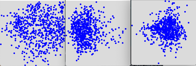
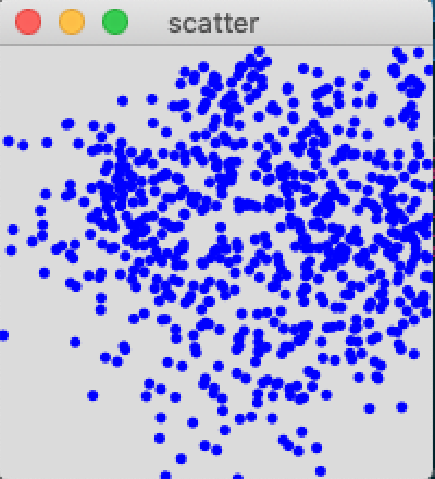
I could start my own thread with this question, but I think it fits in the “PCA…what the?” category. I took a 49 dim spectral shapes stats analysis and used PCA to convert it to two dimensions and 6 dimensions. Why would the first two dimensions of the 6 dimensional plot be exactly the same as the 2 dimensional plot? Pix attached. 2 dim on the top. 6 dim on the bottom in 2 dim clumps.

Yes, I cleared the data before I replotted.

[jamesbradbury]

I’m interested what happens when you reduce to 48. Are the same two dimensions the same? My naive hunch is that PCA does not change much as you go down because those first two dimensions are still captured in the reduction to both 6 and 2. PCA is linear, so maybe those magical orthogonal lines are going through the same points.

[spluta]

Yes. They look the same. I am normalizing, then PCA, then normalizing again.

I guess this is also because the dimensions of the PCA go in order of “differentness”?

Maybe I should be using MDS. Not sure. I want all the dimensions to be equally important. I think.

[tremblap]

IIUC, that is exactly what PCA does! First component is the best approximation, second component is the approximation of the remainder, and so on and so forth…

[weefuzzy]

@spluta

Why would the first two dimensions of the 6 dimensional plot be exactly the same as the 2 dimensional plot?

The tl;dr is because that’s how PCA works: it ‘discovers’ new axes in the space and orders these by how much of the data’s variance each axis accounts for. All that happens when you ask FluidPCA for fewer dimensions is that you get a subset of its internal matrix.

It’s a cheap and cheerful try-this-first (or-as-well) method, rather than a full-blown dimensionality reduction approach. So, if you want equally important dims, yes, try MDS. Or try a gentler PCA to reduce redundancy followed by MDS.

[rodrigo.constanzo]

@rodrigo.constanzo

Ok, I took a stab at “manually” creating a timeness metric.

After all the temporal/morphology talk in the AudioGuide thread I decided to revisit this thread and idea, and wanted to figure out the linear regression stuff anyways.

I shall save you the details of me trying to understand how to implement linear regression in Max, but mercifully one of @Angela’s friends is an MIT’d data scientist, and he held my dumbdumb hand through the process…

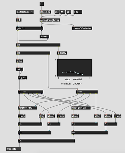
But here is a Max implementation of the slope output of linear regression (based on a translation of this javascript code):

----------begin_max5_patcher----------
10086.3oc68s1aikbcsetmeELB2Oknou06G4SW63DGfXmDD6KLtv3hFTRr0v
YnHEHo5oaGj7aOqUU6CEoDOjEkN5gM7X2pUedtqcser1ONU8e9ce3rKV70Iq
Naze+n+3nO7g+yu6CenbHdfOH+6Ob1Mi+5kyFupbYmM+tatXxxyNudpaGu9x
eX57q+zxIWtt9Xb93GUmOJo9nOoBZsSi+3C4v4i7JdFi4ipQ++kGvh6VOax5
0e61I069ryNezYWLd90ms4RldU4Eu3he76MV08u4kiuYx5IK+zj4iuXV41Ux
4.MNcNdrEJVe+AqurxQM7f+We22webdiC8KWbyMSlutiBVO4qkg7YWMY4zuL
d8zuL4ueC0sbxJbo3fKl+oYSmO4xE2Mub0l94b1j9i9yG4xwO5R1TLF03Opr
2b9nfsv5Taw51luXRm09XW8DF6ed1B7P1LzWNESQ6xz2mnfKUGPgGOfx5mhr
.44WtX1hk0qnHOc+Oz8wchsH074EKuYbgxCGhWdw06P.ly24G2S.Oe4s4S9Y
P9ORb61Q2LY77+sO+q1H1c1QmBzQ+G8XNHDRN7mnMBpUq8GeN.S7jorW1Z3D
D5zaSiSVJCaYbCl+zYS9xjkqf9xVW8GNa7s2t0g+vV2BYV+XcdHc9lCMcd8P
5MGZ4juLs698aN53kfSsFro6VVFom80f6r6eLKfN876lVdR0ChoMgjJSPygX
zpaGeY8l47X2oum26yEgRkqvkCF9Wtr+dtMElls3xeZxUaIGh4famLe57sMg
ryouZxmGe2r0e5yKlud0z+TgBz7gumy+YgB26I4XnP9+BnNOay.35kSuZwbR
D6LSvC2859iiphN5cFLkqX93a2yMC4EvV54jqvf7tUWLdImnDkRS2IWuXwrc
O0l6a1jOuVN8sSmO+Abw0Kts+Stb50+vAt2KVfSdygd1kyr5S2Mud1OAYh0e
Z03urK2d83YyDs3ce7ec77ovXyj0SqSAF0lSVML8Cqtb4hYy1Y7VOyW1yYtB
x3WN4mmd05en7h1VX.W9za6DhNayr7USudxp06dr0iud0tGY05uUY5acn6tP
zg+z5I2b6LLJ18Bf1wzUqW8CK94UxE1InsMC3dTGaqSusIwcN9gLMtq4QZbb
6SrGihUbHVs8wtkr4GZR7PlEg+ooyu253isPp2lR1mUx9bU7gN2EhsmgmOc2
7ebwziwopdo0oxeIXPNJugrkxe5mundB7E6qCe4OMaz0KWb2sMICYhENiWeB
bld4J5XubEyaszx5QWLZ1n+zrKmMY7xlXMZk7WMxaJ.8DImt2S+rJ+6WAn+l
uG.QOtdkmLkBz.mp9OZylS+7D2SP7Q+poTsZ8xIiuYjoMKN1ziwqFhChVl8M
VKq79ZRExU8Ss4mGYX2u419kLT8KYr0Y5h7ca+7kWx7ql70gVLpRCs4BOVcg
mB45+kL8xu1gg7TLendtLj6QJyLBzC9mxXkme+bpUKta4kcy3aLENxryPEf9
VOc9lHG9iaI4OBLkllqNY5fBYiTMQG9WR5n6o2.cDewoC8a+7R2S+3zAQk8B
JenZddw8hSG5loC8K17h6chbZrY4C8K57htY5ne6GxA6RVyYLh7q9TM6CeZ7
50Kmdwcqqld2N6SmTTxWOawEim8fPa2WPze28D2Il4ualrZ03qm7nT+Y8GHU
eVW7iF+9y7tI+PHlG.+vNtJUl8ljOy9Sx2.NVCGZr5Pr6wgerpeiFqN8glWw
f7EXdU8BOVuC.jt6.CKsw+wdFURniGdXwDu7vDMb1z0StYUW3R2MaFO6roqJ
W447GyWve94oKqG6yKK5u6gAoy9ApTS1gK0++cizGmipMoOpBNWJieKqCdqq
MAksSk0trhWZa.8Lbud75I.ZaKi48VeCuqAsiy6QCQmOEqACX8cXrxyld4jC
NtMAIsJ1Opr.6MzbveRF84i791prVOiZ0K7ntupntZ1ha2p.p6wluxVplXz7
3z15zGp7n5T98b4Qi52zxipS+EU4QWOZ1nYG2hgIBGO5f1XLI7mrxkvAed5N
I+YurcfPuUD9poqtc13ucHTDgRJGs5TIg0giON2MEr6NPc+0J+1bkeS05lDS
+0J+9Wq76esxuubU98KS95sKG8+5y5Q+c3mlQ+eVc43YiWRU5Q5ijOYDmaIq
wUG.5XnwRMzWJleGWKlVpOkwWq0at16J4gn.U12urDbcSu4taf5Si7EeguDc
CYyB7dt3u2CopWXUwJrph+nQ4PaRLGrTcuiadBDiFvPr7nUyLTzbr4BnK2PT
+Rcz89UPArkYD2QSLEQGxLHLE+6ZlRKMTRn1E.13GygXz6cvWjSGyCT2kni5
2urn69SSaqmRxpcBUF+ZWUxauAS596CYLVGeJlie85PoYSZqG2zNasN4ChDj
8ctKpQmb2IYhwSqm1NbeIoCu08kzqdyknSl+xq4RL1REWB0v.NdCknS1+hog
RJxvMUf7hW2WrBj2Z4weYohBbq1nizKYabTmULu8zAU2aieD7u37i1jOdI4G
s1bMujsRh9DngWr12nQZ3EU1r0F64kjFHvw1zSi5Wb5P+NfNrMqm9xNuzt8B
2KJcnOI+Z+EcaN0WofSGnNVdWon9tf+wEMsVaK9y8V0pvluWwcJfxlbl+RUb
39FlpCVtN6SdXFeeML2jr482zZkoSaPsmwY7viyz6royFFmNu8zGm42lw4mu
a9kESEGunx6SJ0ntOP6i84Ee98AX+fu8+qmu.utYSu7m1dvsSVId5KI.zt85
e.OaD7TMYEa3oWs3lwSKVISaym2hk5jiN9pqtcwz4qkvuz01sv3xNuKkBAiJ
ES3PmWd57TAqx3zVULn0wP4TV4TwnM3R9PJYcp5obcmRE7ln1FMVsIVNkudJ
swF0JKzg36rblfzzGYky6MrUvTImci6jSTR.NSVeP4.oajrXXjCQPIYqMhwA
aohZMRbGRHn206A8lRy+baBuArqzVNdNjNFsIaXGfgrulaLDZq2F2O+3MpS7
tbwrYils3tqnlx+vcK+B.WbzQ+daDQsNzXK1b9gZ0lf9D5.kNUUNJ9zUiWO9
g.i1r5bDcafDIW1iSnxOM4a6l8ly9x3Y2MYSKWoUdS1pc1jWkqc8DzPSpDTD
yPiTNTf1ExQW1qJFAvgRQm0D7Yn7GkqxGbFCPAnBkbcyCAsKWJ3cdMbpTOjx
nz5jSmBlTbChw8gWUHdceDuIDbJmxa8vvks7zi1rIAaYf7CER.RyYm0yzumS
o5gvjKz4UNsIfY+xghNWH5sVcFBAwxg7wfyaTlHtYlfMZ6RgwM3NjqoBsP6l
9n8nUAiOIvjoMuBsCtdxBalAOXq45grXb.hylwjjWtpXz3MdcJ6TEhW4BF7u
vwv04pyEFmOZvQS.CuOVOjRkBXjji4lHcaejNsbq0YX3OhY+5jpNA1oGzHDG
pzYUlR6yFmxX6jYR3eE8bnKWEbFnf6XSNoMxg73YCrGoP128nzNmCxjIiwZa
g1c8Q6V3pJYiI5CRj2cbr.thG9er0CAla.h6P7FdrqyDNLA.7BfLffbc33ne
wTJacH7m5TnEvITFL8jLYW8FMZWVmsIZSM1Di22qxJTMAqADQBbh5S2FwDO3
fIamBFDqUj6Q1bpprBkPv4Afmrti3gGuTNjvUlwyUtJbDvdfliRDiBTG06wc
B+7MorF5k3AHCf3BFCyf9jI+Xf1OrICNgvsTIXswYrFf4ndHXPwDApAHk6jq
BR5k+oEyFxgTVLApxZXgJ55rZksf23wrsM2BwG6UjO.QVP1zDX0hAsAjALEv
ZfATwlHrFAxhFLDtrN.UhLLAEsZQPBh2V97rzVoXv06vYcUQvyqpXPwGxZYG
LAkZgzS8R5PjA1D0vLi2WsJCm7tXNlbQkJ1MZvbiKjUb5PncKOnAVHyYSry0
.DkgNH7UnBc2HD9ogeusi3gjG3LAHHB6AsP749EZvLLTcfMWuvRMZvYfjcly
HUZvfgBjGhYXqTnAHLDfbiJmywfUzMIS.GFSN5JivjMAXBVawUJOJC88kggR
v2ZxTiV0OmGVfAzRX3.nfENuxGg+vHDCjICMut.Ac4UhrrF7SpCB4oPryQJL
RBYB3rsyDONjGtpyAeRaENeBl2osrLkCah5624JbwDocWH7JS+tnG5bQqI4D
cSewHM0KfCUa2gfZ.lhf0ZQuH.6OPV.5E.OP8pvvKh4OZmRoqJFAiWwuNZ99
bsQ785cElsvrerXJqJj.XGDYKjow+up3A6jv.OD4geoPt5z2PU.LKA6+1pOX
HfCpGiZHxA7fUevH1FSBBc3oKl4wilSMdDkY11FrldcvVrY.oPFfk30GhGVZ
O.1ZjWH35fSooMBXZtdHHXAIohEaw4FjoTkvovHT7uhyCvGYZ1WIZKzDKlYr
zrax2Dw2qGVn.YnmZPdFwuOdiIfXHZ.lAADClF.fKXhv6ko+LvtDBHZwrQ2g
9AWAbgwH0qZAQ9sxPu2P.QzBviwmbFn7Cqw5lH897uhWqEBIfcQnSENCL2AK
OPO.xxv+U4Pf.gAUfJKAemE4AGd2.PQf8AC.8TNDh+EVzQ.Ev8bcP63PDdug
tMB4rKBZ3SzZAqJDai362+pmuKE8jFEjGvaBP.5YzsZQZH.aHFD1qoyMlGZk
vyFDzHbZQLBnG0PMGtuzhleFda8HB23FLRlHiQBNMfzWnIq75dcuhWWFDEbH
AluXM.1jyjQIFlgX.Di8v9tExWUES.DGvmiYHYUCAAdQANXDYBdbNQiVQf8L
qCfv6vYSXfvmFv26aBWftWuqZ5DEVFf1pUfzZIQ.fSQNXDWOdvdSfUCC3BSF
9TCVvpgTQnJXAAHHZSDjfoVCmAXLvPwRf6QIVLLMkfbJPEfoCeaFZ508JS7C
roE4zuOKjJXNFZhP2M2CicIbXvkkXpTz+NTSQbivLeP.CCdokPj5FO3gB0Wf
YEDJBppJzfPFBftYJFLMYnwzenqvFu1Q4c3MpCqMSnGFJ3EJTOPr.y4zyElP
jC4AJNHp3g1tbDP23R.jXWmpBPLRv9.+.FhBNMFFriHFbg1Lwa506JLvCieP
2GPPrUAUfV.gnB4VBrobDvhAVqb.PoPjhEKFH7IH1fvagS+bQdiXrfuHDKYw
rU4FYXi.sMLVB1bU3BQABaV3+AQUSSdWM84cEdDIrCXpFFW7Zg3CzFABbEFr
quQO0kg2TJiWUMvDObv.EVfYIZEevEchH7ACwlJeNCisvSWxQvEaPPXo0VBi
11jwFSedWAjbXB2g.z.T2p+bHglghLzQAWp9FsLeA.4ISObpZuw5YTWN3P.W
SMBFvlQXqvrKHe3Bn9rfsUH8.eAlPcZLQEUlw.X4U2VVC506Jl9LvIJvJgAQ
k2vfvALSelBKUFX.ZdLHDDPdE+.lx.dyXhAzokTkjXzqZ5bF3HD+qvVfSoXB
R5BL.h5IBWE1Ygu1lH9dieM.i5LGQIpG4k2HvC6fodZPP2cHZEmHjAF7tC44
plihwnrAxBb3mIXfTr9rTL+craTCXtUhzAdt3MgW.hPtIpuWGrPmGtWgzCXN
BprLv0iQC9IFEhSIXDDJF9PBQEInLgEIlacljYwmDMxBD8pLAnIyFDCCcbA0
dAIM.S57PfClQazdS+dXM7St0Pi5cAyQ32dlgHDxemHALAwzOAf6QwMOz47P
Dvxgs.Yf1Y.+DBIPMPfySrpdDSF0REvnk7HhwNisoIurl97xBKMvINy6DPyV
sVBTlQl4LPCvrPU+zQXDLGdVJXWQgAamPgMPiel5Q.GFVfTznTMVDnmCQDnI
nYh1hBvLCSKGrRiC0lTeeNYMLJa5v.V200zhBSaNmMCtHrEWw6.G5.uHP9BG
U4JwawrQf4a.QrB6ekCAQPbIr7UvOP01ECC.5uFFhPclEHFfAI5UmkXoIur1
d8xRYDXlrXZTLu.nTH5HEA83DTCv0Y.TkFHxLRb5XDS37ALJcRPe.f.Lp6XX
fVA0umdwcvNuhPsqOdvRXVjMXHzlfis+fX0vTnpDFcJHALXn4.nNxf05xsGr
EloCTfePR7EbymcTzv2kEReQnAZ6v6T2gnAV.8Ci8tPCAuBRj7gSwwlndS+7
dP8YhlEzq7Fo2HBuABlx.hIkJvL4AG.BiFikHGUQl5FQOFxDPyMRgpbmImDi
ROvXwjCQ2FPLB2E700FuuW+rkXEbDlEX9UAS9kB.rIvPBLXJxpfUCdHjuHj+
pxGlIHn.MD8qndfpMhcTiK1H93.3SXgkIVElaqNNLv9OLE.kJXcpsb2X6OJ1
.Quq8TSRB9DTDCsnfU11I1GgAFHp.GTc45vSIsD0tMYQS.bWVzSniDbB.ZXK
FtIBLyHIeWR7yLmEDfmusDz2uiVvsRF.CD74JJgGWh28TZ28TR28TJ2GWB2G
V51lH9PunK8LuiLO8TnthtLCK1vIDvwGjx5DI7FO8rhoJQTx3XZZ.VNls1Jf
SSYrPzkhIT9fwch.sblM4BO4SLG9LRNUa1Ki8R8.eUTQSDIkSLsin+fvIlcA
XDaMU.L86DNQTEqwtTfn.TzAFicUm0UxcXIeCDejLAAT8XPBij5p3EzRbv4L
SQNX8sQ88FNKDYgfKPnAnwYA.nEyCLmq9XGxQOcEv.irvxtXuDz.DiTEeQUY
BLI.QlHyEHtdwZObDiYNHgqSh4X7FwTArgAOMMAxw1a3rHttBHWaDNmpnPxQ
5nBwAgfKpAiCgoDSEHz2fBWEgdIUkDXJqPVMtDJIArDP9AFeDwdBFiH9YAcD
foLbPV6KljmlvI350SKiMRwROSWGgtGObHA6FlMUTH6cvGKf0iHQknpXEerE
XFPfQ.lBGPJBsiZsBoFYUUXjVFopPNFl.A7Cg+1Dbb8GOKcKlYM07RtsfzLU
ig4QaczP2svfIwHPFKOD.4Su+QLUXqxCzoEfCvhWAxudHB5CNj.dB3MoZ5BA
wADpPTC3FZKOBNS+jNjICjTiAUmyRHNCmRHL2XMNHshIpmnOYU+jpAmYHJfN
XV1pAYCmlYBU0wD6UcxlMzjPQyR7gCoyDqUgi08oofYc8lpXhQBAZ.LsLz9Z
ZJfKEn75oWTorCH.WX8LxzMYjPW37SsJPrZtRHUTMFVZY1NkDpXIfGZWO1EU
BznYNIngqfpIEVmq+rmA6kLGEbsPRHBFGNSaO7tHlafHDvCXJ3yDQW5KvpgL
hu1+VkJ6VRMLiC2JLZ.x.3AJVV0cEjiUMAus.igqI3Ytd8xpXvGQJVCa3RHn
fZ.1C3lBFN5ZmBGoM.yJIAiqzNHSnXhercvFzzPukQBiqJ2UfQX9LvqyH0NT
wpSjA6wy+tIpOzeU7A5Rl.CD11lDbwxIPLvHJDohe.Qhp5VM1UpvDq2FKvBB
+UtnXAdIChpq8Pv7UwU.IYc2SGA7lSEy8sUE+9qGKH.CEA.bqt5nE0AlXgDK
HkH8h4BO60i.QSHx3DaKLW6fmTojeTqHBryTeQDbTIKSVFdCQSWM4vrG8eCC
psUcJW+IMlgAArIJ1nLapJL7nC4R3upqeMPfcv+JvPCySRxYgOePlfUlE6kL
I+r1GYFmkoKIqHfd.Ev.GxaFPHDqDc1ZaLuqtd8xFXg.RrJ2bprZQyyzcGX0
h6pfMhMD9fXlBbcoVNyTvlCkDxJjJ44IKqVDhRudHOCDLR.09t5pCzMAOyBJ
KdZSRN9+rtgm785lE9AsLXbVB+tZ5PGgLsZ.1tT5DZviVTfZYWjdUC1vvXW.
tLcMIH2XzwNKnv7OBQfkGDQaJf+fkp.KqLycTSjdutYY2MoIFXij3ZXqApcH
7P1aIUmKTkCVdPjIQoP95J1yLwwzUmDGBijIbNxtaRh+vvFVrjE1t1cBWEio
D7IHzzDo2mSVZFojSI3Bs5PEXNRrx03cRHg0rOUJy.bnh.rq99sTFHfPrTrb
C0DKQNLqdBmHjLfao6AKyTIaVJQ4gk+BJPPcJ1FeuWerDBHadBD3emWJP0FF
9FfRFMccUFydjmUYKJ.+Y30JBYmIBKzkeXCimmsMRrq.yd1uBLfcuDbqkoxk
EmIRWXMQ885iks8EKL.jSjHmS.XCTXiL8oxvgHtfs+To7MR8BzDbOWqACck8
FleBbrvjbH1UTLq44bA2PWSufgOMdB1VihM8mvXl.QMvyifOECkv1A7q.sKL
JDiaL+0vaVTQ9eWzz3dJcsXrq7ZTtIWJbrRJ5bIUqAntB3GVSWcrfF.jhnAz
1JFtuWWrv+MyAVh8Pg.8yBfrZF9Ay.k3QJB0WVQEKr1KS+YB8m0mjl167a4g
9iifBjLFSAP.tAScttlcjtEc7kZXvmMQ885hESfNZY1WhdPxLGqGNfiPTt0i
vTSQG8AaW+HBjNdBvOvjYK7Ybd3oC.WXljE9LQ.CIIH1o6vGfIW1s.vsUSNX
84CHyy5ZpIdWcmoYXZwAFCgrIYUJ.1EafNnwJ43isWG0Byr9ph2T3zjI0mUv
21AcFWigY+SK0Z2.XGL5dDZrps1PHzq+Ul2vngE0FS30nqgyVtJg.CdDtY0l
GBxk8WPjMaSM5ZGSiIBejcc1l1yoTaSnzFEmc34fHdRvjFLEKcsntjVMVfWf
WpIhuW2qvnlwUyYcV5oFXAwvJkvHkjr9B66dpImXtFCcvJskbVyq0zA4B3BJ
hHa.ZvxBxB4CVijQDLu.b3fSQuasw5M8CqzRBQyNAsCaKdi.DSrDaQGwWZ.p
RA8DcXlZS.Cf4VqKJLJTAeRvBlUP1vYqL7kxx9D5BN.Awx1KjVkZh16MNVZV
DJrrOxBRw7KvKMfLKhNhadESd.vumR9t5SwLOoJsAmPVrBC3IgXriR88AdAZ
vgoFRvHQoJVyJD+FdhMQ68mqXV5nDsrDklMCuFEydclcbqTVC1v1rMVYfTcs
YLgfA2vIDtn3zElIgzEhNk0VTZiBLwvJ5BCwQ4PLssNVeDlbnlBFIzqGVl9p
HahFkzMDZlMFZsg4KtJhvldGPHhDFnRPuk0D5KzeMzhSMmrlDyjJ6iZmS5oE
lcJHLAa.ZQwfwk.TM3cZSsUemPn+FGJUj3oGbwsHcwBiHrUI6ZFTBRyyt9vy
RaWsIA.V4D6B.5gndnRn2XZzn55OT.XJCxD3aXRbjBCoXEFMFDXfoME1dcwl
Y7PXxkoVU9NDbr7Tk9IGFD6vDifgJATCDAcL5HatY1H0NYRix7kB9oXMqDUC
fnPw7LAOsB0CsJ9+YJ+ZK8Gg9ihkQNywPhk4SrQvNgfs6zlvSv7.yJPhIuqK
OSEMaLCvDNInAXZgYUSbRIefwF3w0qPrVtz8cNsicFK6Qu17wF5uwhAOoz.2
FSRxTmFRCb0oFZeYaWXffb.hShNSJ9ogIyiE9gx0cYdfMagslz7M2XIHc5ns
KBeCqXESMG8QzT2n2mSVsm3nxkOz.aTpGFndVMb1EAR8crkruR+MDJYsJPIF
0DE6gZinGGJQJB4NeWtu4GWB8Yyp4HoYnzRKvSEKxbakTN1eQYogDc4StKn6
BYvw9qE9ePXacHKKItGGJ2URYKy4jpzWucsjLKEKhZhCBWraFJnY+tx5XroG
qyLdPLL4XqIp2bfDHPiMvD.De5xmWoQafJK+LLDA.N0vCBY8tu1AlVMNAE6Z
bcVDSGMTASIBRBl64RZQ.iVbYyXrXe7lXYsZi56unrrWdXkGcQAgigKpzrMM
H.mp+ELCyVqfIoDNxpxWDtFwAwFdpFLCyoDrmvPs5jufHOaiNhyiUDQLXh.B
Jdwy6ls6m35BvjatntL2tYYk81kStbyZmbX32HS99RaFCYtC7UDV2t2.vzOx
NAFdRKtmKY9JkZ3aHb+e2fp2lOfxFWUxkkmaLm+b14B7p2l0g7GrRGt2wos7
4e5326um8MHKbEaFI89VmCOkA88xRutaWC2u1Edf4UDAziVVGcMrImbn0rvc
G89SXzaGzo76WKBOjf89Vh.d7xR3IMgaealvqK0fx+63h5X19iveEac2R2q6
4bOluXmTt4+J4V3D9lnO32Fs1bBp+ggiw7+dzAWpOD9QBBDkLpjYVprwLaq.
.U53F75eqnGfQdaLq+8iN3p9gqtpe.A9G6CCQ8cbo+CMjSuMC4+1COKGr0gr
kcaI+X2HT4LBLQWVureVSxuQ9t4Fxy8atK6cAMtXJOjfQd9kGFrrYH8ktiwY
eN13T12t8fnCOjqSyuDC4vayP9Hx0cpx6StV2Bxk9Eryucx0G12sOF5cR9Y4
69j1PwdMEqkY4gWrN6daFw2umX72x8DiFF5V.Ti8BQxmR7Ctfs+lVqdhAbkS
uKcLKXQ1qiYc5Y4XN4eW5WFBxkQ7v6WNYem5VVVcxFdk4X9cp4KYR9EXD+9z
obmZ7dcJaSOGo5n8MLQQGIxRtiA56KxRtTq8Lhrbu7hSIfR2qH.Ete88h.PI
pempgKR7CuFdH8dGfR2PeXAnDdp54kG1tK79U1vCWRfElwiWxrspsWJf6cYT
eqkm4Gwxa9cYBM7tLlc1K3O6Gld0UxN12y5suYLbj29tz3hkWU2sHUOuWNyM
TCrY01qW12+x0uFu7Tu7c4H2Lc2EYTWcuy1jdbpzh15lWwAOoKT2Qp70+Jr8
ZO6.w2K6b7uVh2J8q3650SssraLukTYehO6r1l+PgEBJj.g7wOx5rvuROq0Y
CFhVvV2vae74d1TtuEtT1LHboljzxCyLRSRZI+P7tZxrYkhFdKWO3w12KWMD
CzTSBK9g6ccbUJ2fLA95YBrrTI2v6ZPT3RM8thCx7kuIysN6f8tNlrQzbPqs
5x93mGNZcOrfuoRZhe7odtjsK1BKROHS8tc1Gh5c5HNXuK8qz6x1jX1PXWuH
.YOxqZP7Lt6l.Sexy5g5McL1Gi0paWP548lNl.XLODxD5VdULC2Czqx1xqRO
HuJ2wjzUgAaX4O56xNXuqlDAGlW0Q0qFBNXaHiTCh3tJ0765YKD1VPTpgPfO
29q54yBaxKhRMHrvPyuqm63J2hjQdHfL2Tnb4gf+kcs9ld15vsHTj7Cguwle
SOa+8sH7kFBiswbquomK2KzhTdbPFS5VeSO6wTKRDgGa6qlc6w2d6WlrrqOv
KujytY7OtX4lkGeD9y75+rjpxyVN4Ka5a7x2G0YiWd4OLc8jKWe2x5VH2WkM
0mytYwUSVN+toRxJJcs9YqV+sYOLi5a1849E2c0zE+t0iWe2pO8amL+tZp6w
n5yiua15cYEWb8mmNa1kKlUIus628tZBbV8rmuYWfQt1xWnNWFeqKBhbg5JH
qUfF9AKd+1pX8dzc2DWMiTxhhnQV3f3m.i7A59fayb+6heZa00H0tEsAKODK
i412134WW24iLwMa+WrY8Wb6hkcyob0Wby0e25EWub7USksVX0Ncx+4hjzRb
1Baeqc3uytALzoc2y1RdalL9M2c43CMAL9xKwCdGlp03kEvqxJHScs+tdrsF
m6NQvOxDYUrKaSxBzqGd+dvMMY1jad36Kl3mgKuijhKa2key4KKFXaeuqvMW
1qy18t4migr81DkOQ3jRwBpt8MyRYUtuOMcN0VteQNvlMcqFtcxE08Ugce.s
HotYVrGg0FEf1UbMsQHMEU95BtT5wD3CEWCcycA9ew5uUeRuHRqas620I7AC
W+a2NY9ne234qF86lbyzKVL6py1hitC6gej50u.V9cbWWZ6RbARqL16VY.e1
JD+1wqWeHEBN.973Nyy2G9v1aqe+wxF62.QP+6+h0epbapSTOssY3ckA4xzT
cy1vy0aOYIYOU9V814llMAtDt+NkMLuLWlgquSHLxu6rlzwpaycxO19Nd.S0
7mw5aMeaurJb+hkSGO6.5XZY+O3w+ldvjn+C+9+oSTTlK1PxBiDW6upeRcFs
4Ptbzzie01PpaOsJ146+HtbbbIar53OaB0koOeVWVfPOf741EfcC1tck4JKm
Y0OlTsrtDwkDy5WSZ9sW5tMm6u4Xe1uv8+72tZ4hqmL+2WXQ8HiykHQYgqjK
rFxGNtSkGRQ7RGyL8xSTL2IVZ22u0OzpFuomq027QEt68A8DQweuIWq7oay8
dnp6IdHucXDJ2YPj1f26w+1SRT9fRr+5Iym7kw8JqdrA9PJq9K2Z+gc+RrO1
eeZCKVI+1fSV+J5u58FQ8qGOc9+ciTE6p0N+OO92FdRa0OOEJmmjkGsnvd+O
dQnIy6Jh5eY0rorIKNAYqGPMGB.QiFk2eLqsd2OvZwis+Nj7qeyjqNM8v84I
Xe7pvKJYi34VN8qWtd4rmA0OnDD2+qOnwimi.0CDIdUM87ut3ptcT5FrJ1ni
1mE2XOHXFzA7IYB4kVA8e8tat3vDy9r17Xmlu.j1+9zKWebd0SZldPIykSVM
Y86NzF+tKWb6j1gabeVq4dOprt6bPqDupL4e+3KZenznd99jbNp8kAcPgfqt
3n.n2SHe85o7UDIzuew0LTlACN6AlT3dUPT1EmbxB4mSJqxPNj9+dyQJrzqH
68OL9KS97hk27eO3b3SG8n5i9AZvc03k+z2Oe50+v5uujMfSTtu0DMuIqEmX
dT6IEEtMlBhaJlylx5jJu+AHGb5iHtO3IsXvy+1PVhwerLULYoRIeOdCwi5f
wR9vpSbvzZpN.dQ+QDmtuDKO5WFtre0Fs+9VPpmhQbwrIvkYs.f+xEK9oyFH
iS+3sSm+SmZ4xvnT1LLJiZtjf5NPdWa352aztM7Zdj3680xnb41s+si6PngW
4iLy1v8zmJw467yAHOvsSSuh1eG3JY7vD+dLubChZxOUiI6OvV64sFrzLBk3
3Pn2qJ0FO39M1E6l4OTtQTYmzIJYtwPJ+VLMnQ8by3uF32T8oYLJsabKQQV7
4UOmcF+OXhb3.FxAb4Svt8n7LVuIuqeMJ9qG54gcVHS2Og8T3pOaXhoMMnwi
+sCXqJlRxVc2i+sWQW7Om9TaWsi1lEqeJ+mVR21pm9F77ZTWSD9kytax2qO0
VoSGkZQeuMr71VtFRBb4hed9ISgG015.Rg+Cea7oSfJtR0WMRx8QiptCWIzs
COA9qWNYxSfBKbuMohi6Fal3vSb+VXYa95wmL4U1wrksNEkttKxFC4xlQ0PS
i+GSt5jou3Fja5Mw+nDOFCM88+axrYK94SmEZ70lRJl1r6iAoR+wZlMeVoRu
DC.yeNN.Jku3WuX1SPDYSJj7.wjrjqO3ss1s2s71YOMvCwMcSmS6C0UzdtcX
G8GAgpSUAFY7JYWdyvMEtzPNtVN4xIS+xgqb29jY1DXx8iI018W5vPb0PTnX
Qyd7Cb2fJKNBhRmBCo4r8fb6WGonUSle0p2adPtmIO75d6sMiUQYi+KacxVl
F2q2zCpry5w2drN4dqjQ8aFudwneCiB8rA68uZ8jOe2rYqOsBrvOZk59TUXC
Vcl5iG18oOrwFSdecaQi6Sj0cQOtSxXBCKSsNndgFSCX78lTLUA1X2n5X41M
8fZ8b8jUuu9dA9YlMmucpsAPYWXKVSamUlWfxsTkllx6PieuA6Nv4xA2Qxnn
NmUAY6qz3jZsGTp5lrbdmG7V5y+poKW+sQ+iWu3IoNW+z4JUviOyU2JSgk0G
uu6+569e.gJmv1
-----------end_max5_patcher-----------

Here is the relevant code:

function linearRegression(y,x){
        var lr = {};
        var n = y.length;
        var sum_x = 0;
        var sum_y = 0;
        var sum_xy = 0;
        var sum_xx = 0;
        var sum_yy = 0;

        for (var i = 0; i < y.length; i++) {

            sum_x += x[i];
            sum_y += y[i];
            sum_xy += (x[i]*y[i]);
            sum_xx += (x[i]*x[i]);
            sum_yy += (y[i]*y[i]);
        } 

        lr['slope'] = (n * sum_xy - sum_x * sum_y) / (n*sum_xx - sum_x * sum_x);
        lr['intercept'] = (sum_y - lr.slope * sum_x)/n;
        lr['r2'] = Math.pow((n*sum_xy - sum_x*sum_y)/Math.sqrt((n*sum_xx-sum_x*sum_x)*(n*sum_yy-sum_y*sum_y)),2);

        return lr;
}

I also included a vanilla Max version of the mean of the derivative of loudness, to compare the results, along with an option to omit the first frame (which would generally be an uptick).

The included coll dataset has hits from brushes.aif, jongly.aif, and some of my prepared snare stuff, so it’s a cross section of diff types of percussive/drum attacks, and across a fairly wide range of hits, the slope seems to more accurately capture the temporal shape.

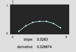
When you have symmetrical samples, the results are pretty much the same:

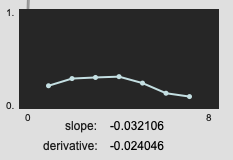
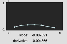
But for things like this, the slope wins out in terms of giving you an idea of what the overall analysis window is doing:

edit:
original screenshots changed since I realized I wasn’t processing the same list of numbers for both.

Although I haven’t implemented it in my code above, there is also the r2 value, which can function in a similar way to the pitch confidence metric, so the higher the r2 value, the tighter the samples fit the slope.

So, I’m thinking of including this as another metric in the timeness descriptor, perhaps also incorporating the r2 as a weighting option for it, so the higher the r2, the more the slope is reflected in the overall timeness value.

@tremblap

this will need all my brains, so not an evening, but a proper three-pipe-problem.

I also imagine that you’re in crunch time leading up to the plenary, but wanted to check on your amountOfPipe-ness as to the overall concept here.